BMS-911543 in vitro CYP1A2 metabolism and time-dependent inactivation (Zhou 2015)

Model and source

• Citation: Zhou L, Gan J, Yoshitsugu H, Gu X, Lutz JD, Masson E, Humphreys WG. Integration of Physiologically-Based Pharmacokinetic Modeling into Early Clinical Development: An Investigation of the Pharmacokinetic Nonlinearity. CPT Pharmacometrics Syst Pharmacol. 2015;4(5):286-294. doi:10.1002/psp4.35. PMCID: PMC4452934. Vmax = 48.1 pmol/min/mg protein and Km = 1.9 uM are the annotations on the ‘HLM kinetics’ panel of Figure 1. Incubation design (0.25 mg/mL human liver microsomes, 1 mM NADPH, pH 7.4 phosphate buffer, 37 C, 10 min, substrate 0.1-10 uM, triplicate, nonlinear fit in GraphPad Prism): Methods, ‘BMS-911543 metabolism’. The fraction unbound in incubation (fumic = 0.78, predicted rather than measured) and the metabolic scaling factor of 4 applied to Km inside the Simcyp model: Methods, ‘PBPK modeling and simulation’. The statement that M1 was the only drug-related component detected in pooled HLM and in cDNA-expressed CYP enzymes, and that CYP1A2 is the primary enzyme with CYP3A4 and CYP2J2 minor: Results, ‘BMS-911543 metabolism’.
• Article: https://doi.org/10.1002/psp4.35
• PubMed Central open-access copy: https://www.ncbi.nlm.nih.gov/pmc/articles/PMC4452934/

This paper contributes five model files, one per in vitro system the authors characterised:

mod_hlm <- rxode2::rxode(readModelDb("Zhou_2015_bms911543_hlm"))
mod_1a2 <- rxode2::rxode(readModelDb("Zhou_2015_bms911543_rcyp1a2"))
mod_3a4 <- rxode2::rxode(readModelDb("Zhou_2015_bms911543_rcyp3a4"))
mod_2j2 <- rxode2::rxode(readModelDb("Zhou_2015_bms911543_rcyp2j2"))
mod_tdi <- rxode2::rxode(readModelDb("Zhou_2015_bms911543_cyp1a2_tdi"))

# Fixed and estimated ini() values are not returned as columns by rxSolve(), so
# read them straight off the packaged model when a check needs one.
ini_val <- function(mod, nm) {
  stopifnot(nm %in% mod$iniDf$name)
  mod$iniDf$est[mod$iniDf$name == nm]
}

Scope: what this paper does and does not contribute

Zhou 2015 has two halves, and only one of them is reproducible.

The first half is the authors’ own bench work: a Michaelis-Menten characterisation of the formation of metabolite M1 from BMS-911543 in pooled human liver microsomes and in three recombinant CYP systems (Figure 1), and a mechanism-based inactivation study of CYP1A2 by the same compound using phenacetin O-deethylation as the activity probe (Figure 2). Both fitted equations are printed, every constant is printed, the incubation designs are described in the Methods, and the two studies are the reverse-translation step the paper is written around: they were run because the first physiologically based model, built on the pre-clinical package, could not reproduce the dose-dependent and time-dependent nonlinearity BMS-911543 showed in its first-in-human study. That is the layer this vignette validates and that the five model files carry.

The second half is a Simcyp V12 whole-body physiologically based model that consumes those constants to simulate plasma profiles across nine dose levels. That layer is a vendor platform model and is not extracted. The paper reports no tissue volumes, no organ blood flows, no MPPGL, no liver weight and no hepatic CYP abundances; the whole-body ODE system is Simcyp’s rather than the authors’; and no project file is deposited. Reconstructing it would require substituting physiology from outside the source, which is exactly the substitution the library’s PBPK sourcing rule forbids. The section “Published results not reproduced here” below records what that half produced, so a reader can see precisely what was left on the table and why.

Two consequences of that split are load-bearing for the in vitro layer and are called out where they arise:

• The authors deliberately changed two of the in vitro constants when they moved them into the platform model, to close an in-vitro-to-in-vivo gap. A metabolic scaling factor of 4 was applied to every Km (entered as Km/4), and the CYP1A2 inactivation constant KI was raised from the measured 2.9 uM to 11.2 uM. The model files carry the measured values, because they are the in vitro models. The paper’s own Discussion concedes that the two adjusted inputs “are not identifiable”.
• Three quantities the platform half needed are not in the source at all: the CYP1A2 degradation rate constant kdeg (the authors used the Simcyp default and never print it), and the maximal fold induction and EC50 of CYP1A2 autoinduction (taken from Supplementary Table S3, which is not on disk). Nothing in the five model files depends on them.

In vitro systems

In vitro systems of Zhou 2015 (Methods).

Assay	System	Buffer	Design	Readout	Fit
M1 formation kinetics	Pooled human liver microsomes at 0.25 mg/mL, and cDNA-expressed recombinant CYP1A2, CYP3A4 and CYP2J2 (enzyme content not reported)	pH 7.4 phosphate, 1 mM NADPH, 37 C	10 min incubation; BMS-911543 0.1-10 uM; triplicate	M1 formation velocity by LC/MS/MS	Nonlinear fitting, GraphPad Prism
CYP1A2 inactivation	Human liver microsomes at 1.0 mg/mL	100 mM potassium phosphate pH 7.4, 1 mM NADPH, 37 C	5 min preincubation, then 3, 10, 20 or 30 min inactivation without phenacetin; 10-fold dilution into 450 uM phenacetin for 13.5 min; BMS-911543 0 to 25 uM; triplicate	Acetaminophen formation from phenacetin, as percent of the no-inhibitor control	Nonlinear regression, GraphPad Prism v.5

The two assays run at different microsomal protein concentrations, 0.25 and 1.0 mg/mL, so their fractions unbound in incubation are not interchangeable and only the metabolism arm has a reported one.

The clinical study that motivated the work is a first-in-human open-label dose escalation in patients with cancer (NCT01236352): 5 to 240 mg across nine dose levels, a single dose on day 1 followed by a 24 h washout, then twice-daily dosing for two weeks; 833 plasma timepoints from 72 subjects. No population PK model is reported for it – the only clinical parameter the paper prints is a “preliminary population PK analysis” estimate of Vss/F of about 50 L – so there is no clinical model to extract either.

Source trace

Every value in the five model files, with the location it came from.

Source trace for every ini() value and every model equation.

Model	Quantity	Value	Source location
Zhou_2015_bms911543_hlm	km_hlm	1.9 uM	Figure 1, ‘HLM kinetics’ panel annotation
Zhou_2015_bms911543_hlm	vmax_hlm	48.1 pmol/min/mg protein	Figure 1, ‘HLM kinetics’ panel annotation
Zhou_2015_bms911543_hlm	prot_inc (fixed)	0.25 mg/mL	Methods, ‘BMS-911543 metabolism’
Zhou_2015_bms911543_hlm	fumic (fixed)	0.78	Methods, ‘PBPK modeling and simulation’ (Simcyp built-in PREDICTION, not measured)
Zhou_2015_bms911543_rcyp1a2	km_cyp1a2	2.1 uM	Figure 1, ‘CYP1A2 kinetics’ panel annotation
Zhou_2015_bms911543_rcyp1a2	vmax_cyp1a2	3.2 pmol/min/pmol protein	Figure 1, ‘CYP1A2 kinetics’ panel annotation
Zhou_2015_bms911543_rcyp3a4	km_cyp3a4	1.4 uM	Figure 1, ‘CYP3A4 kinetics’ panel annotation
Zhou_2015_bms911543_rcyp3a4	vmax_cyp3a4	0.048 pmol/min/pmol protein	Figure 1, ‘CYP3A4 kinetics’ panel annotation
Zhou_2015_bms911543_rcyp2j2	km_cyp2j2	1.3 uM	Figure 1, ‘CYP2J2 kinetics’ panel annotation
Zhou_2015_bms911543_rcyp2j2	vmax_cyp2j2	0.5 pmol/min/pmol protein	Figure 1, ‘CYP2J2 kinetics’ panel annotation
Zhou_2015_bms911543_cyp1a2_tdi	ki_1a2	2.9 uM	Figure 2b annotation and Results, ‘CYP1A2 TDI by BMS-911543’ (2.9 +/- 0.9 uM)
Zhou_2015_bms911543_cyp1a2_tdi	kinact_1a2	1.4 /h	Figure 2b annotation and Results, ‘CYP1A2 TDI by BMS-911543’ (1.4 +/- 0.1 per h)
all five	addSd (fixed at 0)	0	Not reported anywhere in the source; see Assumptions
Michaelis-Menten form	v = Vmax*S/(Km+S)	-	Methods, ‘BMS-911543 metabolism’; the fitted curves of Figure 1
Inactivation form (Eq. 1)	vI = v0exp(-kt)	-	Methods, ‘CYP1A2 time-dependent inhibition’
Inactivation form (Eq. 2)	k = kinact*I/(KI+I)	-	Methods, ‘CYP1A2 time-dependent inhibition’

All eight Michaelis-Menten constants live in the annotations of Figure 1, not in any table or in the body text. The Results section says only that “the observed enzyme kinetic values for Vmax and Km are listed in Figure 1”. Those annotations are rendered text inside the figure image and are therefore invisible to a PDF-to-text converter; they were read off the rendered figure panel. The values are printed by the authors and are not digitised measurements from the plotted points, so their precision is the authors’ own, but the reading step is recorded here as non-text provenance.

Dimensional analysis

The one unit bridge in the package, in the human liver microsome model, is worth checking explicitly. Getting it wrong misstates every rate by a factor of 1000 and nothing else in the model catches it.

# Vmax [pmol/(min*mg protein)] * protein [mg/mL] = pmol/(min*mL)
#   1 pmol/mL = 1 nmol/L = 0.001 umol/L = 0.001 uM,  hence the /1000.
vmax_hlm <- ini_val(mod_hlm, "vmax_hlm")
km_hlm   <- ini_val(mod_hlm, "km_hlm")
prot_inc <- ini_val(mod_hlm, "prot_inc")

rate_at_vmax_uM_per_min <- vmax_hlm * prot_inc / 1000
c(vmax_pmol_min_mg = vmax_hlm, protein_mg_mL = prot_inc,
  max_rate_uM_per_min = rate_at_vmax_uM_per_min)
#>    vmax_pmol_min_mg       protein_mg_mL max_rate_uM_per_min 
#>           48.100000            0.250000            0.012025

# Vmax/Km with Vmax in pmol/min/mg and Km in uM (= pmol/uL) is uL/min/mg.
c(clint_hlm_uL_min_mg = vmax_hlm / km_hlm)
#> clint_hlm_uL_min_mg 
#>            25.31579

Simulation grid

The in vitro “cohort” is a grid of incubation concentrations, not a set of subjects; there is no inter-individual variability anywhere in this paper. The grids below are well under the 200-per-arm cap.

# Log-spaced concentrations spanning the 0.1-10 uM experimental range of the
# metabolism assay, plus an exact point at each system's own Km.
conc_grid <- sort(unique(c(
  0,
  exp(seq(log(0.05), log(20), length.out = 60)),
  ini_val(mod_1a2, "km_cyp1a2"),
  ini_val(mod_3a4, "km_cyp3a4"),
  ini_val(mod_2j2, "km_cyp2j2"),
  km_hlm,
  10
)))
length(conc_grid)
#> [1] 66

Replicating Figure 1: Michaelis-Menten kinetics of M1 formation

The three recombinant models are static concentration-response models and solve from a one-row-per-concentration frame. The human liver microsome model is an ODE, so its initial velocity is read at time zero after dosing the substrate into the incubation.

solve_static <- function(mod, grid) {
  rxode2::rxSolve(
    mod,
    data.frame(id = seq_along(grid), time = 0, CP_BMS911543_UM = grid),
    returnType = "data.frame"
  ) |>
    dplyr::transmute(conc = CP_BMS911543_UM, velocity = vM1)
}

# The HLM model is dosed: the substrate is spiked into the incubation at t = 0,
# so the initial velocity is vM1 on the t = 0 record. Observation rows are placed
# on the `bms911543` ODE state, never on the algebraic observable.
ev_hlm_initial <- do.call(rbind, lapply(seq_along(conc_grid), function(i) {
  rbind(
    data.frame(id = i, time = 0, amt = conc_grid[i], evid = 1L, cmt = "bms911543"),
    data.frame(id = i, time = 0, amt = NA_real_,     evid = 0L, cmt = "bms911543")
  )
}))

hlm_initial <-
  rxode2::rxSolve(mod_hlm, ev_hlm_initial, returnType = "data.frame") |>
  dplyr::transmute(conc = Cbms911543, velocity = vM1)
#> Warning: multi-subject simulation without without 'omega'

fig1 <- dplyr::bind_rows(
  dplyr::mutate(hlm_initial,                  panel = "HLM (pmol/min/mg protein)"),
  dplyr::mutate(solve_static(mod_1a2, conc_grid), panel = "rCYP1A2 (pmol/min/pmol protein)"),
  dplyr::mutate(solve_static(mod_3a4, conc_grid), panel = "rCYP3A4 (pmol/min/pmol protein)"),
  dplyr::mutate(solve_static(mod_2j2, conc_grid), panel = "rCYP2J2 (pmol/min/pmol protein)")
)
#> Warning: multi-subject simulation without without 'omega'
#> Warning: multi-subject simulation without without 'omega'
#> Warning: multi-subject simulation without without 'omega'

ggplot2::ggplot(fig1, ggplot2::aes(conc, velocity)) +
  ggplot2::geom_line(linewidth = 0.7) +
  ggplot2::facet_wrap(~panel, scales = "free_y") +
  ggplot2::coord_cartesian(xlim = c(0, 15)) +
  ggplot2::labs(x = "Substrate concentration (uM)", y = "M1 formation velocity") +
  ggplot2::theme_bw()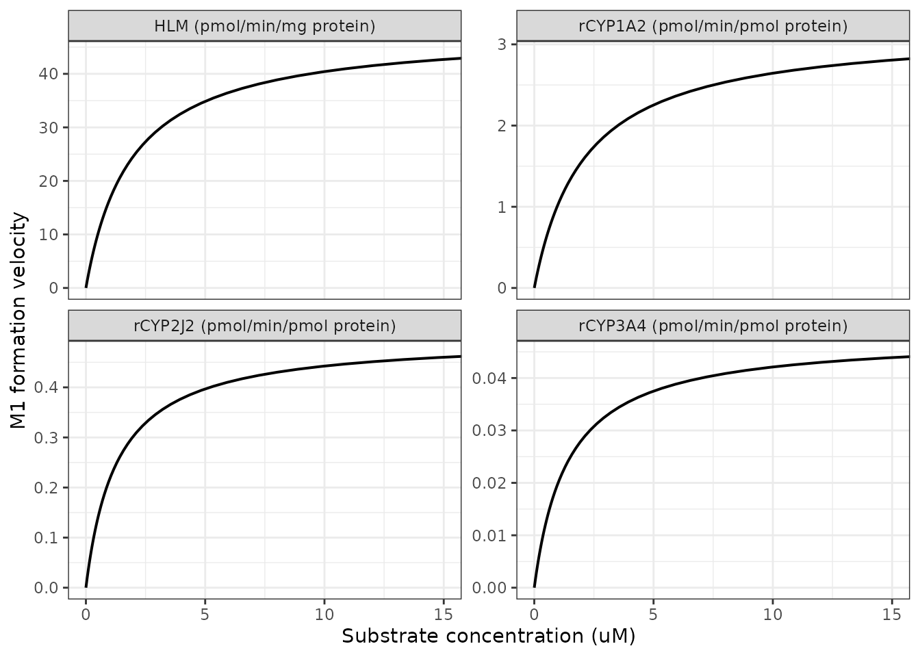

Replicates Figure 1 of Zhou 2015: M1 formation velocity against BMS-911543 concentration in pooled human liver microsomes and in three recombinant CYP systems. Each panel has its own velocity scale, as in the source.

Structural identities

These hold exactly, from the printed constants alone, and are the strongest available check that the eight Figure 1 annotations were transcribed correctly into the right slots: a Km and a Vmax swapped between panels, or a decimal point moved, breaks them immediately.

mm_check <- function(mod, km_name, vmax_name, label) {
  km   <- ini_val(mod, km_name)
  vmax <- ini_val(mod, vmax_name)
  got  <- solve_static(mod, c(0, km, 1e6))
  tibble::tibble(
    system         = label,
    km             = km,
    vmax           = vmax,
    v_at_zero      = got$velocity[1],
    v_at_km        = got$velocity[2],
    half_vmax      = vmax / 2,
    v_at_infinity  = got$velocity[3],
    clint          = vmax / km
  )
}

mm <- dplyr::bind_rows(
  mm_check(mod_1a2, "km_cyp1a2", "vmax_cyp1a2", "rCYP1A2"),
  mm_check(mod_3a4, "km_cyp3a4", "vmax_cyp3a4", "rCYP3A4"),
  mm_check(mod_2j2, "km_cyp2j2", "vmax_cyp2j2", "rCYP2J2")
)
#> Warning: multi-subject simulation without without 'omega'
#> Warning: multi-subject simulation without without 'omega'
#> Warning: multi-subject simulation without without 'omega'

stopifnot(
  # No substrate, no product.
  all(mm$v_at_zero == 0),
  # The defining property of the Michaelis constant.
  all(abs(mm$v_at_km - mm$half_vmax) < 1e-10),
  # The velocity saturates at Vmax.
  all(abs(mm$v_at_infinity - mm$vmax) / mm$vmax < 1e-4)
)

# The same three identities in the dosed HLM model.
hlm_id <- rxode2::rxSolve(
  mod_hlm,
  do.call(rbind, lapply(seq_along(c(km_hlm, 1e6)), function(i) {
    s <- c(km_hlm, 1e6)[i]
    rbind(data.frame(id = i, time = 0, amt = s,          evid = 1L, cmt = "bms911543"),
          data.frame(id = i, time = 0, amt = NA_real_,   evid = 0L, cmt = "bms911543"))
  })),
  returnType = "data.frame"
)
#> Warning: multi-subject simulation without without 'omega'
stopifnot(
  abs(hlm_id$vM1[1] - vmax_hlm / 2) < 1e-8,
  abs(hlm_id$vM1[2] - vmax_hlm) / vmax_hlm < 1e-4
)

knitr::kable(mm, digits = 4, caption = "Michaelis-Menten structural identities in the three recombinant systems.")

Michaelis-Menten structural identities in the three recombinant systems.

system	km	vmax	v_at_zero	v_at_km	half_vmax	v_at_infinity	clint
rCYP1A2	2.1	3.200	0	1.600	1.600	3.200	1.5238
rCYP3A4	1.4	0.048	0	0.024	0.024	0.048	0.0343
rCYP2J2	1.3	0.500	0	0.250	0.250	0.500	0.3846

Coarse cross-check against the plotted points

The Figure 1 panels also carry the measured points the curves were fitted to. These were read off the rendered figure and are not a source of any model value; they are recorded here only to confirm that the curve the model draws is the curve the source drew, at the concentration where the panels are easiest to read. The tolerance is deliberately loose, because the uncertainty here is in the reading, not in the model.

digitised_at_10uM <- tibble::tribble(
  ~panel_source,          ~observed_read_off_figure,
  "HLM",                  38.5,
  "rCYP1A2",              2.75,
  "rCYP3A4",              0.0465,
  "rCYP2J2",              0.44
)

predicted_at_10uM <- tibble::tibble(
  panel_source = c("HLM", "rCYP1A2", "rCYP3A4", "rCYP2J2"),
  predicted = c(
    vmax_hlm * 10 / (km_hlm + 10),
    ini_val(mod_1a2, "vmax_cyp1a2") * 10 / (ini_val(mod_1a2, "km_cyp1a2") + 10),
    ini_val(mod_3a4, "vmax_cyp3a4") * 10 / (ini_val(mod_3a4, "km_cyp3a4") + 10),
    ini_val(mod_2j2, "vmax_cyp2j2") * 10 / (ini_val(mod_2j2, "km_cyp2j2") + 10)
  )
)

cmp10 <- dplyr::left_join(predicted_at_10uM, digitised_at_10uM, by = "panel_source") |>
  dplyr::mutate(pct_diff = 100 * (observed_read_off_figure - predicted) / predicted)

# Centre and spread, not the extreme of the four readings.
stopifnot(
  abs(median(cmp10$pct_diff)) < 15,
  max(abs(cmp10$pct_diff)) < 30
)

knitr::kable(cmp10, digits = 4,
             caption = "Model velocity at 10 uM against the topmost plotted point of each Figure 1 panel, read off the rendered figure.")

Model velocity at 10 uM against the topmost plotted point of each Figure 1 panel, read off the rendered figure.

panel_source	predicted	observed_read_off_figure	pct_diff
HLM	40.4202	38.5000	-4.7505
rCYP1A2	2.6446	2.7500	3.9844
rCYP3A4	0.0421	0.0465	10.4375
rCYP2J2	0.4425	0.4400	-0.5600

Cross-system comparison

Two free comparisons the source makes itself, reproduced from the packaged constants.

cross <- tibble::tibble(
  system = c("HLM", "rCYP1A2", "rCYP3A4", "rCYP2J2"),
  km_uM  = c(km_hlm, ini_val(mod_1a2, "km_cyp1a2"),
             ini_val(mod_3a4, "km_cyp3a4"), ini_val(mod_2j2, "km_cyp2j2")),
  vmax   = c(vmax_hlm, ini_val(mod_1a2, "vmax_cyp1a2"),
             ini_val(mod_3a4, "vmax_cyp3a4"), ini_val(mod_2j2, "vmax_cyp2j2"))
) |>
  dplyr::mutate(clint = vmax / km_uM)

# 1. All four Michaelis constants sit inside a narrow band, consistent with one
#    dominant binding mode for the reaction across the four systems.
km_spread <- max(cross$km_uM) / min(cross$km_uM)
stopifnot(km_spread < 2)

# 2. The three recombinant systems share a per-pmol-enzyme denominator, so their
#    Vmax/Km values are directly comparable and must rank CYP1A2 first, which is
#    the paper's own reaction-phenotyping conclusion ("CYP1A2 was the primary
#    enzyme mediating the formation of M1 ... CYP3A4 and CYP2J2 played a minor
#    role", Results).
rec <- dplyr::filter(cross, system != "HLM")
stopifnot(
  rec$system[which.max(rec$clint)] == "rCYP1A2",
  rec$system[which.min(rec$clint)] == "rCYP3A4"
)

c(km_fold_spread = km_spread,
  clint_1a2_over_2j2 = rec$clint[rec$system == "rCYP1A2"] / rec$clint[rec$system == "rCYP2J2"],
  clint_1a2_over_3a4 = rec$clint[rec$system == "rCYP1A2"] / rec$clint[rec$system == "rCYP3A4"])
#>     km_fold_spread clint_1a2_over_2j2 clint_1a2_over_3a4 
#>           1.615385           3.961905          44.444444

knitr::kable(cross, digits = 4,
             caption = "Michaelis constants and per-system intrinsic clearances. The HLM clint is uL/min/mg microsomal protein; the three recombinant clints are uL/min/pmol enzyme and are comparable only with each other.")

Michaelis constants and per-system intrinsic clearances. The HLM clint is uL/min/mg microsomal protein; the three recombinant clints are uL/min/pmol enzyme and are comparable only with each other.

system	km_uM	vmax	clint
HLM	1.9	48.100	25.3158
rCYP1A2	2.1	3.200	1.5238
rCYP3A4	1.4	0.048	0.0343
rCYP2J2	1.3	0.500	0.3846

Note what this comparison cannot do. Turning the per-enzyme ranking into a fraction metabolised requires the hepatic abundance of each isoform, an intersystem extrapolation factor and MPPGL, none of which the source reports. The Simcyp model’s predicted 96 percent fraction metabolised by CYP1A2 is therefore a platform output, not something reproducible here, and it is listed below rather than asserted.

The human liver microsome incubation as a dynamic system

Because the microsomal protein concentration of the metabolism assay is reported, that one arm supports a full substrate-depletion ODE. Two exact checks follow from it.

# The concentrations the authors used, over the 10 min incubation of the Methods.
s0 <- c(0.1, 0.2, 0.5, 1, 2, 5, 10)
ev_hlm <- do.call(rbind, lapply(seq_along(s0), function(i) {
  rbind(
    data.frame(id = i, time = 0, amt = s0[i], evid = 1L, cmt = "bms911543"),
    data.frame(id = i, time = seq(0, 10, by = 0.25), amt = NA_real_, evid = 0L, cmt = "bms911543")
  )
}))

hlm_run <- rxode2::rxSolve(mod_hlm, ev_hlm, returnType = "data.frame") |>
  dplyr::mutate(s0 = s0[id])
#> Warning: multi-subject simulation without without 'omega'

Mass balance. The only routes in the model are substrate to M1, so the sum of the two states must equal the spiked concentration at every time, exactly.

mb <- hlm_run |>
  dplyr::mutate(total = bms911543 + m1,
                rel_err = abs(total - s0) / s0)
stopifnot(max(mb$rel_err) < 1e-8)
c(max_relative_mass_balance_error = max(mb$rel_err))
#> max_relative_mass_balance_error 
#>                     1.24345e-15

Initial-rate conditions. The Methods report a single 10 min incubation and fit initial-rate Michaelis-Menten kinetics to it, which is only valid if substrate depletion stays small. The model says by how much, at every concentration the authors used – and the worst case is the lowest concentration, because that is where the fractional turnover is largest.

depletion <- hlm_run |>
  dplyr::filter(time == 10) |>
  dplyr::transmute(s0, remaining = bms911543,
                   pct_consumed = 100 * (s0 - bms911543) / s0)

# The conventional initial-rate criterion is under 20 percent turnover.
stopifnot(max(depletion$pct_consumed) < 20)

knitr::kable(depletion, digits = 4,
             caption = "Substrate consumed over the 10 min human liver microsome incubation, by starting concentration.")

Substrate consumed over the 10 min human liver microsome incubation, by starting concentration.

s0	remaining	pct_consumed
0.1	0.0942	5.8437
0.2	0.1888	5.5799
0.5	0.4754	4.9117
1.0	0.9591	4.0902
2.0	1.9388	3.0600
5.0	4.9131	1.7385
10.0	9.8990	1.0097

ggplot2::ggplot(hlm_run, ggplot2::aes(time, bms911543 / s0, group = factor(s0), colour = factor(s0))) +
  ggplot2::geom_line(linewidth = 0.7) +
  ggplot2::scale_y_continuous(limits = c(0.9, 1)) +
  ggplot2::labs(x = "Incubation time (min)", y = "Fraction of spiked substrate remaining",
                colour = "Spiked (uM)") +
  ggplot2::theme_bw()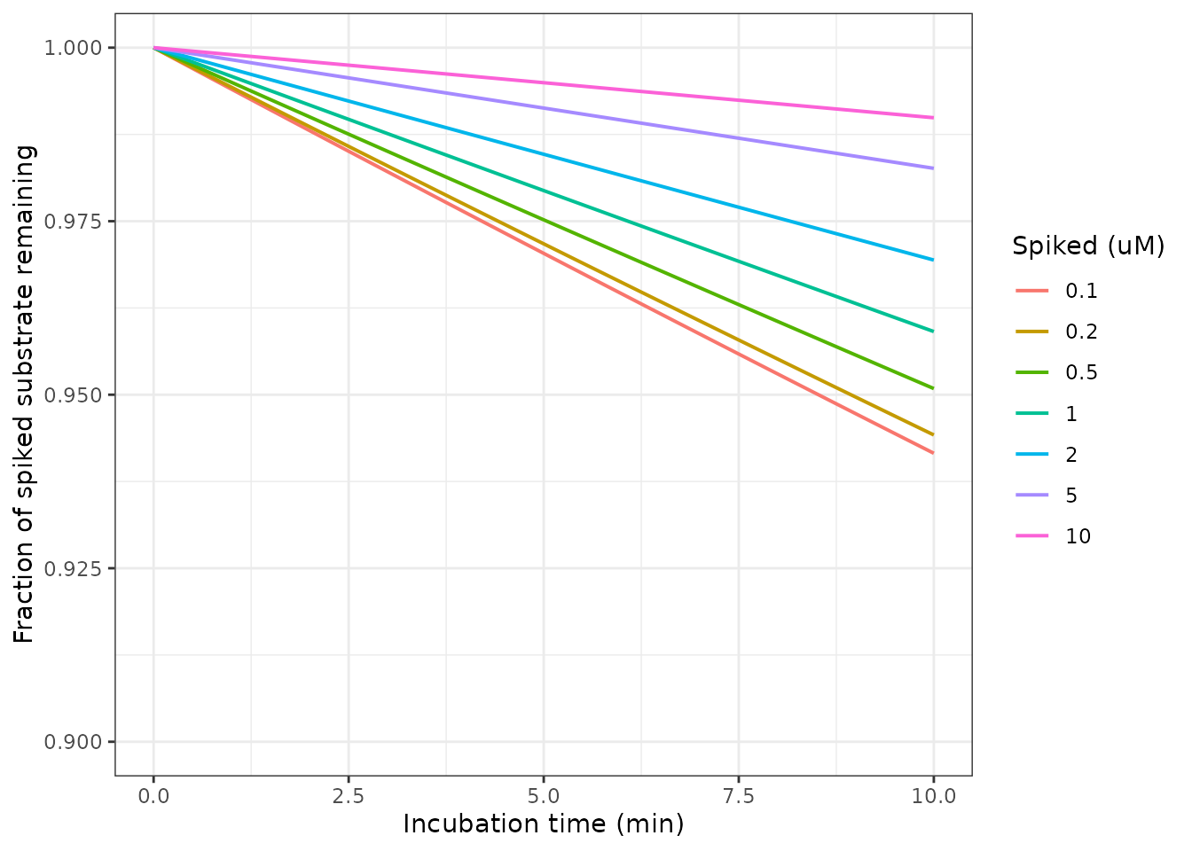

Substrate depletion over the 10 min human liver microsome incubation of Zhou 2015 Methods. The initial-rate assumption behind the Figure 1 fit holds at every concentration used.

Replicating Figure 2: time-dependent inactivation of CYP1A2

The inactivation model runs on an hour timescale, because the reported kinact is in per-hour units while the assay times are in minutes.

inh_conc <- c(0, 0.39, 0.78, 1.56, 3.125, 6.25, 12.5, 25.0)   # Methods
tdi_times_min <- seq(0, 30, by = 0.5)

ev_tdi <- do.call(rbind, lapply(seq_along(inh_conc), function(i) {
  data.frame(id = i, time = tdi_times_min / 60, CP_BMS911543_UM = inh_conc[i])
}))

tdi_run <- rxode2::rxSolve(mod_tdi, ev_tdi, returnType = "data.frame") |>
  dplyr::mutate(time_min = time * 60, inhibitor = CP_BMS911543_UM)
#> Warning: multi-subject simulation without without 'omega'

ggplot2::ggplot(tdi_run,
                ggplot2::aes(time_min, pctActivity_1a2,
                             group = factor(inhibitor), colour = factor(inhibitor))) +
  ggplot2::geom_line(linewidth = 0.7) +
  ggplot2::scale_y_log10(limits = c(50, 140)) +
  ggplot2::labs(x = "Preincubation time (min)", y = "Percent CYP1A2 activity remaining",
                colour = "BMS-911543 (uM)") +
  ggplot2::theme_bw()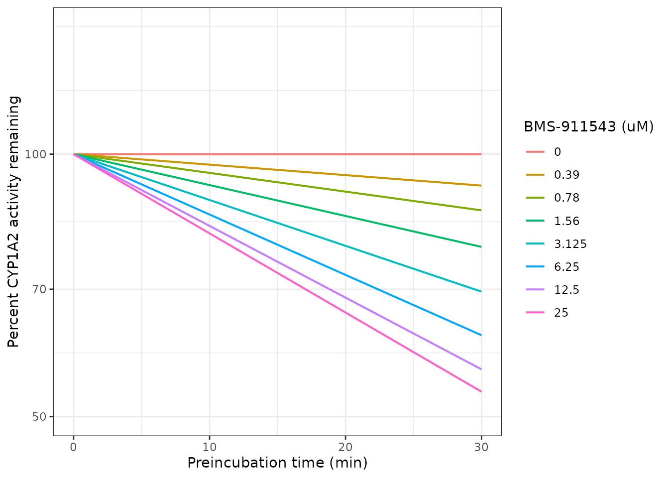

Replicates Figure 2a of Zhou 2015: percent CYP1A2 activity remaining against preincubation time, one line per BMS-911543 concentration, on a log activity scale.

lambda_curve <- rxode2::rxSolve(
  mod_tdi,
  data.frame(id = seq_len(101), time = 0,
             CP_BMS911543_UM = seq(0, 30, length.out = 101)),
  returnType = "data.frame"
)
#> Warning: multi-subject simulation without without 'omega'

ggplot2::ggplot(lambda_curve,
                ggplot2::aes(CP_BMS911543_UM, lambda_1a2_permin)) +
  ggplot2::geom_line(linewidth = 0.7) +
  ggplot2::coord_cartesian(ylim = c(0, 0.03)) +
  ggplot2::labs(x = "BMS-911543 concentration (uM)",
                y = "Inactivation rate constant lambda (1/min)") +
  ggplot2::theme_bw()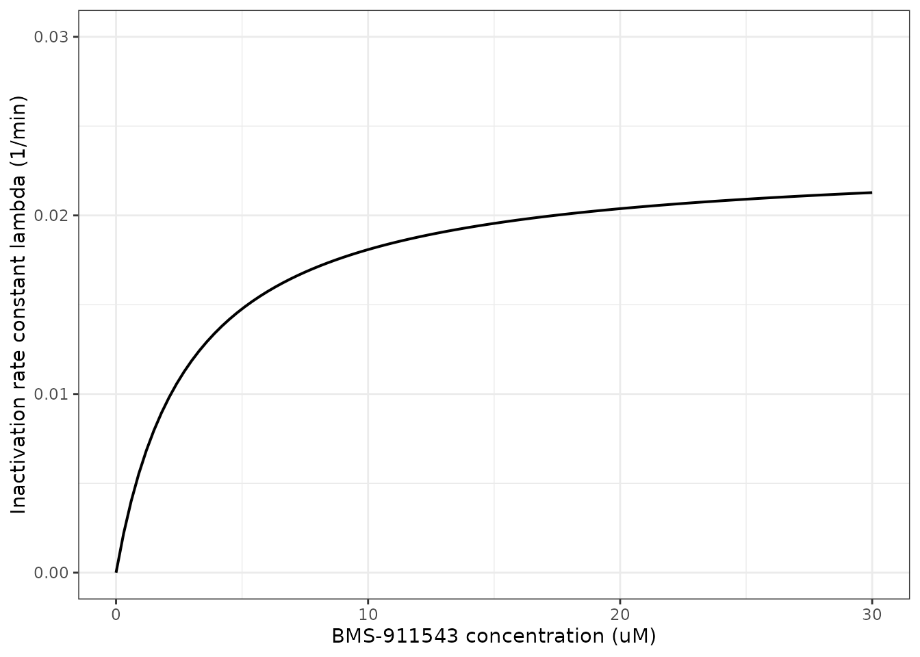

Replicates Figure 2b of Zhou 2015: the first-order inactivation rate constant against the initial BMS-911543 concentration, plotted in the source’s per-minute units.

Structural identities of the inactivation model

ki     <- ini_val(mod_tdi, "ki_1a2")
kinact <- ini_val(mod_tdi, "kinact_1a2")

probe <- rxode2::rxSolve(
  mod_tdi,
  data.frame(id = 1:3, time = 0, CP_BMS911543_UM = c(0, ki, 1e7)),
  returnType = "data.frame"
)
#> Warning: multi-subject simulation without without 'omega'

stopifnot(
  # Eq. 2 at I = 0: no inhibitor, no inactivation.
  probe$kobs_1a2[1] == 0,
  # The defining property of KI: half the maximum rate of inactivation.
  abs(probe$kobs_1a2[2] - kinact / 2) < 1e-10,
  # The plateau of Figure 2b is kinact.
  abs(probe$kobs_1a2[3] - kinact) / kinact < 1e-5,
  # Eq. 1 at I = 0: the no-inhibitor control holds at 100 percent for all time.
  all(tdi_run$pctActivity_1a2[tdi_run$inhibitor == 0] == 100)
)

# Eq. 1 is a first-order decay, so the ODE solution must equal exp(-k*t) to
# solver tolerance at every concentration and every time. This is the check that
# the ODE encoding of the published closed form is faithful.
closed_form <- tdi_run |>
  dplyr::mutate(analytic = exp(-kobs_1a2 * time),
                abs_err = abs(enzyme_1a2 - analytic))
stopifnot(max(closed_form$abs_err) < 1e-6)
c(max_abs_error_vs_published_closed_form = max(closed_form$abs_err))
#> max_abs_error_vs_published_closed_form 
#>                           2.766371e-07

Coarse cross-check against Figure 2

As with Figure 1, these readings come off the rendered figure and are used only to confirm the model draws the curve the source drew.

# Readings taken from the FITTED CURVE of Figure 2b (more legible than the
# scattered points) and from the lowest line of Figure 2a at 30 min.
lambda_at_25 <- lambda_curve$lambda_1a2_permin[which.min(abs(lambda_curve$CP_BMS911543_UM - 25))]
lambda_at_25_read <- 0.0205

activity_at_25_30min <- tdi_run$pctActivity_1a2[tdi_run$inhibitor == 25 & tdi_run$time_min == 30]
activity_at_25_30min_read <- 57

tibble::tibble(
  quantity = c("lambda at 25 uM (1/min), Figure 2b curve",
               "percent activity at 25 uM and 30 min, Figure 2a"),
  model = c(lambda_at_25, activity_at_25_30min),
  read_off_figure = c(lambda_at_25_read, activity_at_25_30min_read)
) |>
  knitr::kable(digits = 4, caption = "Model against readings from the Figure 2 panels.")

Model against readings from the Figure 2 panels.

quantity	model	read_off_figure
lambda at 25 uM (1/min), Figure 2b curve	0.0209	0.0205
percent activity at 25 uM and 30 min, Figure 2a	53.4064	57.0000

stopifnot(
  abs(lambda_at_25 - lambda_at_25_read) < 0.005,
  abs(activity_at_25_30min - activity_at_25_30min_read) < 10
)

The Figure 2a reading sits a few percentage points above the model. That is expected rather than a discrepancy: the lines of Figure 2a are the individual log-linear regressions at each concentration, whereas the model’s rate constant comes from the hyperbola fitted through all of them in Figure 2b, and the two need not coincide at any single concentration.

Why there is no NCA section

PKNCA validation is not applicable to this package. None of the five models has a dosing route, a volume of distribution or a plasma concentration-time profile: four are enzyme-kinetic velocity models of a microsomal or recombinant incubation, and the fifth is an enzyme-inactivation model whose state is a dimensionless activity fraction. The equivalent checks for this model class – dimensional analysis, mass balance, structural identities and agreement with the published closed form – are the sections above.

Published results not reproduced here

Everything below is an output of the Simcyp V12 whole-body model, which is not extracted. It is recorded so a reader can see the full scope of the paper and what would be needed to close each gap.

Published results of the platform half of Zhou 2015, and why each is out of scope.

Published result	Value	Why it is not reproduced
Fraction of BMS-911543 metabolised by CYP1A2	96 percent of total clearance	Needs hepatic abundances of CYP1A2, CYP3A4 and CYP2J2, an intersystem extrapolation factor and MPPGL. None is reported.
Absorption rate constant	ka = 4.138 /h	A Simcyp ADAM absorption-model output; the underlying solubility, particle-size and gastrointestinal transit inputs are in Supplementary Tables S1 and S3, which are not on disk.
Fraction of dose absorbed	Fa falls from 1 to 0.42 over 5-240 mg	Same as above; the dose-dependence is a solubility-limited absorption prediction of the platform model.
Fraction escaping gut-wall metabolism	Fg = 1	A platform output; no intestinal physiology is reported.
Adjusted apparent clearance	Falls from 11.3 to 7.3 L/h over the dose range	Derived as Fa * dose / AUC(day 1) using the platform’s own Fa and the observed AUCs of Figure 4; both inputs are unavailable as numbers.
Hepatic CYP1A2 activity remaining at day 15	62 percent with induction, 54 percent without, so induction attenuates the inactivation by 17 percent	Requires the enzyme degradation rate constant kdeg (Simcyp default, never printed), the autoinduction Emax and EC50 (Supplementary Table S3, not on disk), and a liver unbound-concentration profile from the whole-body model.
Volume of distribution at steady state	0.26 L/kg (18.2 L at 70 kg) from rat tissue-to-plasma ratios; about 2 L/kg from in silico partition coefficients	The rat tissue distribution study’s partition coefficients are not tabulated in the paper, and no whole-body physiology is reported to combine them with.
Clinical population PK	Vss/F about 50 L, described as a preliminary analysis	A single parameter with no clearance, no absorption and no structural model; not an extractable model.
Clinical half-life by dose	2.0-2.8 h at 5-40 mg; 2.7-5.7 h at 80-240 mg	Non-compartmental summaries of the first-in-human study, reported without the underlying concentration data (Supplementary Table S2 is not on disk).

Assumptions and deviations

• The Simcyp V12 whole-body PBPK model is not extracted. The paper reports no tissue volumes, no organ blood flows, no MPPGL, no liver weight and no hepatic CYP abundances; the whole-body ODEs belong to the platform; and no project file is deposited. Reconstructing it would require importing physiology from outside the source. The table above records what that half produced.
• The measured KI of 2.9 uM is carried, not the 11.2 uM used in the platform model. The authors substituted the higher value to fit the clinical data and say so explicitly, giving a best-fit clinical value of 11 +/- 3.4 uM in the Discussion and conceding that Km and KI “are not identifiable”. These are the in vitro models, so they carry the in vitro measurement. A user who wants the platform’s behaviour should set ki_1a2 to 11.2.
• The metabolic scaling factor of 4 is not applied. Inside the platform model every Km was entered as Km/4 to close an in-vitro-to-in-vivo extrapolation gap, a fitting device chosen by “the best fitting to the FIH day 1 plasma concentration data”. The Km values here are the ones Figure 1 reports.
• All eight Michaelis-Menten constants were read off the Figure 1 panel annotations, because the source reports them nowhere else – the Results text says only that they are “listed in Figure 1”. They are the authors’ printed values, not digitised from the plotted points, but the reading step is non-text provenance and is recorded as such in the source-trace table.
• No residual-error model, and no variability of any kind, is reported. The source fitted every curve in GraphPad Prism and reports point estimates only. Per the standing policy on unreported residual error, addSd is fixed(0) in all five files, so each model returns the deterministic published curve. The +/- 0.9 uM and +/- 0.1 per h printed alongside the inactivation constants are standard errors of the nonlinear regression, not between-subject or between-donor variability, and are deliberately not encoded as an omega. No SE is printed for any of the eight Michaelis-Menten constants.
• The recombinant models are static velocity models, not depletion ODEs. The recombinant CYP content of those incubations is not reported – the 0.25 mg/mL in the same Methods sentence is the human liver microsome protein concentration – so a volumetric rate cannot be formed without inventing a number. The published fit is the velocity curve, so the static form is also the faithful one. The human liver microsome model does carry the depletion ODE, because its protein concentration is reported. This asymmetry between siblings is deliberate and reflects exactly what each arm of the source supports.
• fumic = 0.78 is a Simcyp prediction, not a measurement. The paper says it “was predicted to be 0.78 using the built-in method”. It is carried fixed() in the human liver microsome model so the unbound Michaelis constant is visible and auditable, and so a user with a measured value can override it. Nothing in the Figure 1 fit depends on it.
• The CYP1A2 autoinduction arm is absent. Its maximal fold induction and EC50 were taken from experimental values reported in Supplementary Table S3, which is not on disk. That supplement is immaterial to everything extracted here: all eight metabolism constants are in Figure 1 and both inactivation constants are in Figure 2 and in the Results text.
• No enzyme resynthesis term. The inactivation model describes the inactivation limb of a microsomal assay, in which no enzyme is made. Extending it to the in-vivo turnover balance would need kdeg, which the authors say they took from the Simcyp default and never print.
• The observation-name convention warning is accepted, not silenced. checkModelConventions() warns that the four metabolism models’ single output vM1 is not the canonical Cc. The endpoint is a reaction velocity in pmol/min per mg or per pmol of protein; renaming it to Cc would misstate its units and falsify the units$concentration metadata. This is the same disposition taken for vUK408027 in Hyland_2008_maraviroc_hlm.R. The inactivation model has no such warning: its output is the registered canonical compartment enzyme_1a2.
• The digitised figure readings are cross-checks only. No model value comes from them, the assertions on them are on the centre and a loose bound rather than on any single extreme reading, and each is labelled at the point of use.

Session information

sessionInfo()
#> R version 4.6.1 (2026-06-24)
#> Platform: x86_64-pc-linux-gnu
#> Running under: Ubuntu 24.04.5 LTS
#> 
#> Matrix products: default
#> BLAS:   /usr/lib/x86_64-linux-gnu/openblas-pthread/libblas.so.3 
#> LAPACK: /usr/lib/x86_64-linux-gnu/openblas-pthread/libopenblasp-r0.3.26.so;  LAPACK version 3.12.0
#> 
#> locale:
#>  [1] LC_CTYPE=C.UTF-8       LC_NUMERIC=C           LC_TIME=C.UTF-8       
#>  [4] LC_COLLATE=C.UTF-8     LC_MONETARY=C.UTF-8    LC_MESSAGES=C.UTF-8   
#>  [7] LC_PAPER=C.UTF-8       LC_NAME=C              LC_ADDRESS=C          
#> [10] LC_TELEPHONE=C         LC_MEASUREMENT=C.UTF-8 LC_IDENTIFICATION=C   
#> 
#> time zone: UTC
#> tzcode source: system (glibc)
#> 
#> attached base packages:
#> [1] stats     graphics  grDevices utils     datasets  methods   base     
#> 
#> other attached packages:
#> [1] ggplot2_4.0.3         tidyr_1.3.2           dplyr_1.2.1          
#> [4] rxode2_5.1.8          nlmixr2lib_0.3.2.9000
#> 
#> loaded via a namespace (and not attached):
#>  [1] generics_0.1.4      sass_0.4.10         xml2_1.6.0         
#>  [4] digest_0.6.39       magrittr_2.0.5      RColorBrewer_1.1-3 
#>  [7] evaluate_1.0.5      grid_4.6.1          fastmap_1.2.0      
#> [10] lotri_1.0.5         jsonlite_2.0.0      whisker_0.4.1      
#> [13] rxode2ll_2.0.18     backports_1.5.1     purrr_1.2.2        
#> [16] scales_1.4.0        textshaping_1.0.5   jquerylib_0.1.4    
#> [19] cli_3.6.6           crayon_1.5.3        symengine_0.2.13   
#> [22] rlang_1.3.0         withr_3.0.3         cachem_1.1.0       
#> [25] yaml_2.3.12         otel_0.2.0          tools_4.6.1        
#> [28] parallel_4.6.1      memoise_2.0.1       checkmate_2.3.4    
#> [31] rxode2lincmt_0.1.0  vctrs_0.7.3         R6_2.6.1           
#> [34] lifecycle_1.0.5     fs_2.1.0            ragg_1.5.2         
#> [37] PreciseSums_0.7     fontawesome_0.5.3   pkgconfig_2.0.3    
#> [40] desc_1.4.3          rex_1.2.2           pkgdown_2.2.1      
#> [43] pillar_1.11.1       bslib_0.12.0        gtable_0.3.6       
#> [46] glue_1.8.1          data.table_1.18.6.1 Rcpp_1.1.2         
#> [49] systemfonts_1.3.2   tidyselect_1.2.1    xfun_0.61          
#> [52] tibble_3.3.1        sys_3.4.3           knitr_1.52         
#> [55] farver_2.1.2        dparser_1.3.1-13    htmltools_0.5.9    
#> [58] labeling_0.4.3      rmarkdown_2.32      compiler_4.6.1     
#> [61] S7_0.2.2            downlit_0.4.5       askpass_1.2.1      
#> [64] openssl_2.4.2