Enalapril and enalaprilat, serum and urine (Faisal 2019) • nlmixr2lib

Model and source

Faisal 2019 fitted a single simultaneous semi-mechanistic population PK model to four data streams at once – serum enalapril, serum enalaprilat, cumulative urinary enalapril and cumulative urinary enalaprilat – from a two-period crossover in 24 healthy adults. The paper reports three fits, and all three are packaged here:

Model	Source table	Data
`Faisal_2019_enalapril`	Table 1	both periods pooled, with a formulation covariate on MTT1
`Faisal_2019_enalapril_reference`	Supplementary Table Supp-I	reference-tablet period only
`Faisal_2019_enalapril_odmt`	Supplementary Table Supp-II	ODMT period only

The pooled model is the paper’s primary result. The two formulation-specific fits are the paper’s second, co-primary analysis strategy (Methods, “Population Pharmacokinetic Modeling Strategy”, item 2): they exist so that the individual parameter estimates from each formulation could be compared subject-by-subject with a paired Wilcoxon signed-rank test. They are not robustness checks, and the ODMT fit is structurally distinct (six absorption transit compartments rather than eight).

Citation: Faisal M, Cawello W, Burckhardt BB, de Hoon J, Laer S; LENA Consortium. Simultaneous Semi-Mechanistic Population Pharmacokinetic Modeling Analysis of Enalapril and Enalaprilat Serum and Urine Concentrations From Child Appropriate Orodispersible Minitablets. Front Pediatr. 2019;7:281. doi:10.3389/fped.2019.00281
Article: https://doi.org/10.3389/fped.2019.00281
Supplementary material (Tables Supp-I and Supp-II): https://www.frontiersin.org/articles/10.3389/fped.2019.00281/full#supplementary-material
Companion paper on the same trial (individual-fit Bateman analysis, used below as an external check): Faisal M, Cawello W, Laer S. Drug Des Devel Ther 2019;13:481-90, https://doi.org/10.2147/DDDT.S188417

cat(strwrap(rxode2::rxode2(readModelDb("Faisal_2019_enalapril"))$description, 78), sep = "\n")
#> ℹ parameter labels from comments will be replaced by 'label()'
#> Simultaneous semi-mechanistic population PK model for the prodrug enalapril
#> and its active diacid metabolite enalaprilat, fitted jointly to serum
#> concentrations AND cumulative urinary excretion amounts of both analytes in
#> 24 healthy adults given a single 10 mg oral dose of enalapril maleate (Faisal
#> 2019, LENA consortium). Enalapril absorption is an 8-compartment Erlang
#> transit chain (rate ktr) feeding the central compartment at rate ka;
#> enalapril leaves the central compartment by two parallel first-order routes,
#> direct urinary excretion (kurine) and metabolic conversion to enalaprilat
#> (kmet). The enalaprilat formation phase is delayed by a 2-compartment Erlang
#> transit chain (rate ktr_enaat) before entering a two-compartment enalaprilat
#> disposition model that is eliminated only by urinary excretion
#> (kurine_enaat). Cumulative urinary amounts of both analytes are carried as
#> explicit excretion compartments, which is what makes the absolute
#> bioavailability F1 identifiable (estimated 0.606). Body weight scales the
#> enalapril central volume with the exponent FIXED at 1 and referenced to the
#> study mean 69.76 kg; the orodispersible-minitablet formulation multiplies the
#> enalapril mean transit time by 0.730 relative to the reference tablet. DOSE
#> BASIS: supply the dose as the LABELLED mass of enalapril MALEATE (the trial's
#> 10 mg = 10000 ug), not as enalapril free base. This differs from
#> Steichert_2025_enalapril_enalaprilat_pediatric.R, which requires free base;
#> to move a dose between the two models multiply or divide by 376.45/492.52 =
#> 0.76433.

Population

Twenty-four healthy adult volunteers took part in a two-treatment, two-period crossover phase I relative-bioavailability trial (NCT02252692) run within the EU FP7 LENA project (Labeling of Enalapril from Neonate to Adolescence). In each period a single 10 mg oral dose of enalapril maleate was given with 240 mL of water: as two 5 mg market-authorised conventional tablets (Renitec, the reference) in one period, and as ten 1 mg child-appropriate orodispersible minitablets (ODMTs) in the other.

Baseline demographics (Table 2) were: age mean 28.00 years (median 24.40, range 22.08-47.16), weight mean 69.76 kg (median 67.60, range 51.8-95.6), height mean 174.5 cm (range 153.0-189.0) and total body water mean 42.06 L (range 32.86-53.70). The analysis dataset held 2,208 serum and urine concentrations. Serum was sampled at 0.17, 0.33, 0.5, 0.75, 1, 1.25, 1.5, 2, 2.5, 3, 3.5, 4, 4.5, 5, 6, 8, 10, 12, 24 and 48 h; urine was collected over 0-2, 2-4, 4-8, 8-12, 12-24, 24-36 and 36-48 h and converted to cumulative excreted amounts.

The same information is available programmatically via the model’s population metadata (readModelDb() returns the model function, so the trailing () evaluates it):

str(readModelDb("Faisal_2019_enalapril")()$population, max.level = 1)
#> List of 16
#>  $ species               : chr "human"
#>  $ n_subjects            : num 24
#>  $ n_studies             : num 1
#>  $ age_range             : chr "22.08-47.16 years"
#>  $ age_mean              : chr "28.00 years"
#>  $ age_median            : chr "24.40 years"
#>  $ weight_range          : chr "51.8-95.6 kg"
#>  $ weight_mean           : chr "69.76 kg"
#>  $ weight_median         : chr "67.60 kg"
#>  $ height_range          : chr "153.0-189.0 cm"
#>  $ total_body_water_range: chr "32.86-53.70 L"
#>  $ race_ethnicity        : NULL
#>  $ disease_state         : chr "Healthy adult volunteers"
#>  $ dose_range            : chr "Single 10 mg oral dose of enalapril maleate in each of two periods (two-treatment, two-period crossover). Refer"| __truncated__
#>  $ regions               : chr "Belgium (University Hospitals Leuven / KU Leuven)"
#>  $ notes                 : chr "Demographics from Table 2. Phase I relative-bioavailability trial NCT02252692 within the EU FP7 LENA project (L"| __truncated__

Model structure

Figure 1 of the paper gives the schematic, which the model file reproduces state-for-state:

dose --F1--> transit1 -> ... -> transit8 --KA--> central (enalapril, VC)
                                                   |  \
                                          KREN     |   \  KM
                                                   v    v
                                                 urine   transit1_enaat -> transit2_enaat
                                                                                |
                                                                                v
              peripheral1_enaat <--KQ1/KQ2--> central_enaat (enalaprilat, VM)
                                                   |
                                          KMEL     v
                                              urine_enaat

Three features are worth calling out.

The urine compartments are what make F1 identifiable. The paper assumes enalapril is eliminated only by urinary excretion (KREN) and by conversion to enalaprilat (KM), and that enalaprilat is eliminated only by urinary excretion (KMEL) and is not metabolised further. With both serum and cumulative urinary amounts fitted, the system closes and absolute bioavailability becomes estimable rather than confounded with volume. The estimate, F1 = 0.606, matches the literature value of ~60% absorbed.

Absorption and metabolite formation are both Erlang transit chains. A lag-time model failed to describe the low concentrations at the onset of each phase, so transit compartments were added stepwise. The paper prints MTT = (N + 1) / KTR in both the Methods text and Figure 1, and estimates KA separately as the transfer out of the last transit; the model file uses that convention exactly as written.

Only the mean transit time differs between formulations. In the pooled model the formulation enters through Equation 7, TV = theta_X * theta_12^FORM * exp(eta), on MTT1 alone.

Source trace

Every ini() entry in the model files carries an in-file comment naming its origin. Collected here for the pooled model (Faisal_2019_enalapril):

Equation / parameter	Value	Source location
Structure (compartments, arrows)	–	Figure 1; Methods “Population Pharmacokinetic Model Structure”
`MTT = (N + 1) / KTR`	–	Methods text; Figure 1 annotation
Transit counts N = 8, N = 2	–	Results (“Eight transits … for reference and pooled data analysis”); Figure 1
BSV model `Pi = TVp * exp(ETAi)`	–	Equation 3
Residual error (serum add+prop, urine prop)	–	Equations 4 and 5; Methods “Population Pharmacokinetic Model Structure”
Weight on VC	`(WT/69.76)^1`	Equation 6; Table 2 (mean weight); Results “Model Evaluation Results”
Formulation on MTT1	`0.730^FORM`	Equation 7; Table 1 row “THETA (X)”
`lka` (KA)	6.010 1/h	Table 1
`lvc` (VC)	51.10 L	Table 1
`lfdepot` (F1)	0.606	Table 1
`lmtt` (MTT1)	0.558 h	Table 1
`lkurine` (KREN)	0.305 1/h	Table 1
`lkmet` (KM)	0.688 1/h	Table 1
`lvc_enaat` (VM)	46.10 L	Table 1
`lk12_enaat` (KQ1)	0.060 1/h	Table 1
`lk21_enaat` (KQ2)	0.054 1/h	Table 1
`lkurine_enaat` (KME)	0.184 1/h	Table 1
`lmtt_enaat` (MTT2)	0.910 h	Table 1
`etal*` (9 IIV variances)	0.041-0.688	Table 1, “INTERINDIVIDUAL VARIABILITY (IIV)”
`propSd`, `addSd`, `propSd_enaat`, `addSd_enaat`, `propSd_urineEna`, `propSd_urineEnaat`	see model file	Table 1, “RESIDUAL UNEXPLAINED VARIABILITY (RUV)”

The two formulation-specific model files trace to Supplementary Tables Supp-I and Supp-II respectively, parameter for parameter.

Typical-value profiles

The paper reports no concentration-time table, but its Results section makes two quantitative claims about the typical profile that a correct implementation must reproduce: enalapril reaches Cmax in “almost 1 h” and enalaprilat in “around 3 to 4 h”.

Because the model declares four endpoints, typical-value solves use omega = NA, sigma = NA rather than zeroRe(), and useLinCmt = FALSE.

Note on the event tables below: observation rows carry cmt = "Cc", naming the algebraic observable rather than an ODE state. For a single-endpoint model that would be wrong – it injects a compartment slot and renumbers the states – but this model declares four endpoints, and rxode2 then requires observation records to resolve to a declared endpoint: cmt = "central" and cmt = NA both fail with 'dvid'->'cmt' or 'cmt' on observation record or on a undefined compartment. Here the four observables are appended as slots 16-19 behind the fifteen ODE states, doses are placed by name (cmt = "transit1") rather than by number, and every solve returns all four outputs. The exact mass-balance check below is the independent proof that nothing was renumbered.

doseUg <- 10000 # 10 mg enalapril maleate, as labelled (see Errata)
wtRef <- 69.76

mPooled <- rxode2::rxode2(readModelDb("Faisal_2019_enalapril"))
#> ℹ parameter labels from comments will be replaced by 'label()'

solveTypical <- function(model, form = NULL, tmax = 72, by = 0.02) {
  ev <- rxode2::et(amt = doseUg, cmt = "transit1") |>
    rxode2::et(seq(0, tmax, by = by), cmt = "Cc")
  ev <- as.data.frame(ev)
  ev$WT <- wtRef
  if (!is.null(form)) ev$FORM_ODMT <- form
  rxode2::rxSolve(
    model, ev,
    returnType = "data.frame", useLinCmt = FALSE,
    omega = NA, sigma = NA, atol = 1e-10, rtol = 1e-10
  )
}

typ <- bind_rows(
  solveTypical(mPooled, form = 0) |> mutate(treatment = "Reference tablet"),
  solveTypical(mPooled, form = 1) |> mutate(treatment = "ODMT")
)

typ |>
  group_by(treatment) |>
  summarise(
    `Enalapril Cmax (ug/L)` = max(Cc),
    `Enalapril Tmax (h)` = time[which.max(Cc)],
    `Enalaprilat Cmax (ug/L)` = max(Cc_enaat),
    `Enalaprilat Tmax (h)` = time[which.max(Cc_enaat)],
    .groups = "drop"
  ) |>
  knitr::kable(digits = 2)

treatment	Enalapril Cmax (ug/L)	Enalapril Tmax (h)	Enalaprilat Cmax (ug/L)	Enalaprilat Tmax (h)
ODMT	78.93	0.72	55.97	3.14
Reference tablet	75.82	0.88	55.88	3.26

tmaxEna <- typ |> filter(treatment == "Reference tablet") |> summarise(t = time[which.max(Cc)]) |> pull(t)
tmaxEnaat <- typ |> filter(treatment == "Reference tablet") |> summarise(t = time[which.max(Cc_enaat)]) |> pull(t)

# Deterministic (typical-value) solve, so tight bounds are appropriate here:
# these are numerical properties of the published parameters, not draws.
stopifnot(
  # Results: enalapril Cmax "achieved in almost 1 h".
  tmaxEna > 0.5, tmaxEna < 1.5,
  # Results: enalaprilat Cmax "in around 3 to 4 h".
  tmaxEnaat > 2.5, tmaxEnaat < 4.5
)

Both Tmax values land where the paper says they do, and both Cmax values sit comfortably below the assay upper limits of quantification (200 ng/mL for enalapril, 188 ng/mL for enalaprilat), as they must for the reported calibration ranges to have been fit for purpose.

typ |>
  select(time, treatment, Enalapril = Cc, Enalaprilat = Cc_enaat) |>
  pivot_longer(c(Enalapril, Enalaprilat), names_to = "Analyte", values_to = "conc") |>
  filter(time <= 24) |>
  ggplot(aes(time, conc, colour = treatment, linetype = Analyte)) +
  geom_line(linewidth = 0.8) +
  labs(x = "Time (h)", y = "Serum concentration (ug/L)", colour = NULL, linetype = NULL) +
  theme_bw()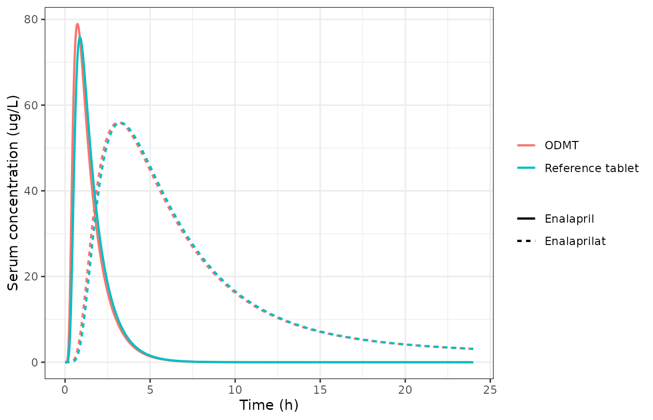

Typical-value serum profiles of enalapril and enalaprilat after a single 10 mg oral dose of enalapril maleate, by formulation. Reproduces the median behaviour of the VPC panels A and C of Figure 3 of Faisal 2019.

The enalaprilat curves for the two formulations are visually indistinguishable, which is the paper’s central conclusion: the formulation changes when the prodrug appears, and nothing about the active metabolite.

Mass balance: an exact closed-form gate

The model’s elimination assumptions make the ultimate urinary recovery an exact algebraic quantity, independent of every absorption parameter. All absorbed drug (F1 * Dose) must eventually appear in urine, split between the two enalapril exit routes in proportion to their rate constants:

total recovered = F1 * Dose
as enalapril = F1 * Dose * KREN / (KREN + KM)
as enalaprilat = F1 * Dose * KM / (KREN + KM)

This is a genuine structural check: a transposed rate constant, a wrong bioavailability target compartment, or a missing arrow all break it.

thPooled <- rxode2::rxode2(readModelDb("Faisal_2019_enalapril"))$theta
#> ℹ parameter labels from comments will be replaced by 'label()'
kurine <- exp(thPooled[["lkurine"]])
kmet <- exp(thPooled[["lkmet"]])
fdepot <- exp(thPooled[["lfdepot"]])

expTotal <- fdepot * doseUg
expEna <- expTotal * kurine / (kurine + kmet)
expEnaat <- expTotal * kmet / (kurine + kmet)

# Solve far past the terminal phase so the slow enalaprilat peripheral
# compartment has emptied (KQ2 = 0.054 1/h implies a ~13 h half-life).
long <- solveTypical(mPooled, form = 0, tmax = 400, by = 0.5)
obs <- long[nrow(long), ]

data.frame(
  Quantity = c("Total in urine", "As enalapril", "As enalaprilat"),
  `Closed form (ug)` = c(expTotal, expEna, expEnaat),
  `Simulated (ug)` = c(obs$urineEna + obs$urineEnaat, obs$urineEna, obs$urineEnaat),
  check.names = FALSE
) |>
  mutate(`% diff` = 100 * (`Simulated (ug)` - `Closed form (ug)`) / `Closed form (ug)`) |>
  knitr::kable(digits = c(0, 1, 1, 3))

Quantity	Closed form (ug)	Simulated (ug)
Total in urine	6060.0	6060.0
As enalapril	1861.3	1861.3
As enalaprilat	4198.7	4198.7

# Deterministic identity: tolerance is numerical, not biological.
stopifnot(
  abs(obs$urineEna + obs$urineEnaat - expTotal) / expTotal < 1e-3,
  abs(obs$urineEna - expEna) / expEna < 1e-3,
  abs(obs$urineEnaat - expEnaat) / expEnaat < 1e-3
)

The split reproduces to better than 0.1%: 30.7% of the absorbed dose leaves as unchanged enalapril and 69.3% as enalaprilat.

typ |>
  filter(treatment == "Reference tablet", time <= 48) |>
  select(time, Enalapril = urineEna, Enalaprilat = urineEnaat) |>
  pivot_longer(c(Enalapril, Enalaprilat), names_to = "Analyte", values_to = "amt") |>
  ggplot(aes(time, amt, colour = Analyte)) +
  geom_line(linewidth = 0.8) +
  geom_hline(yintercept = c(expEna, expEnaat), linetype = "dashed", linewidth = 0.3) +
  labs(x = "Time (h)", y = "Cumulative amount in urine (ug)", colour = NULL) +
  theme_bw()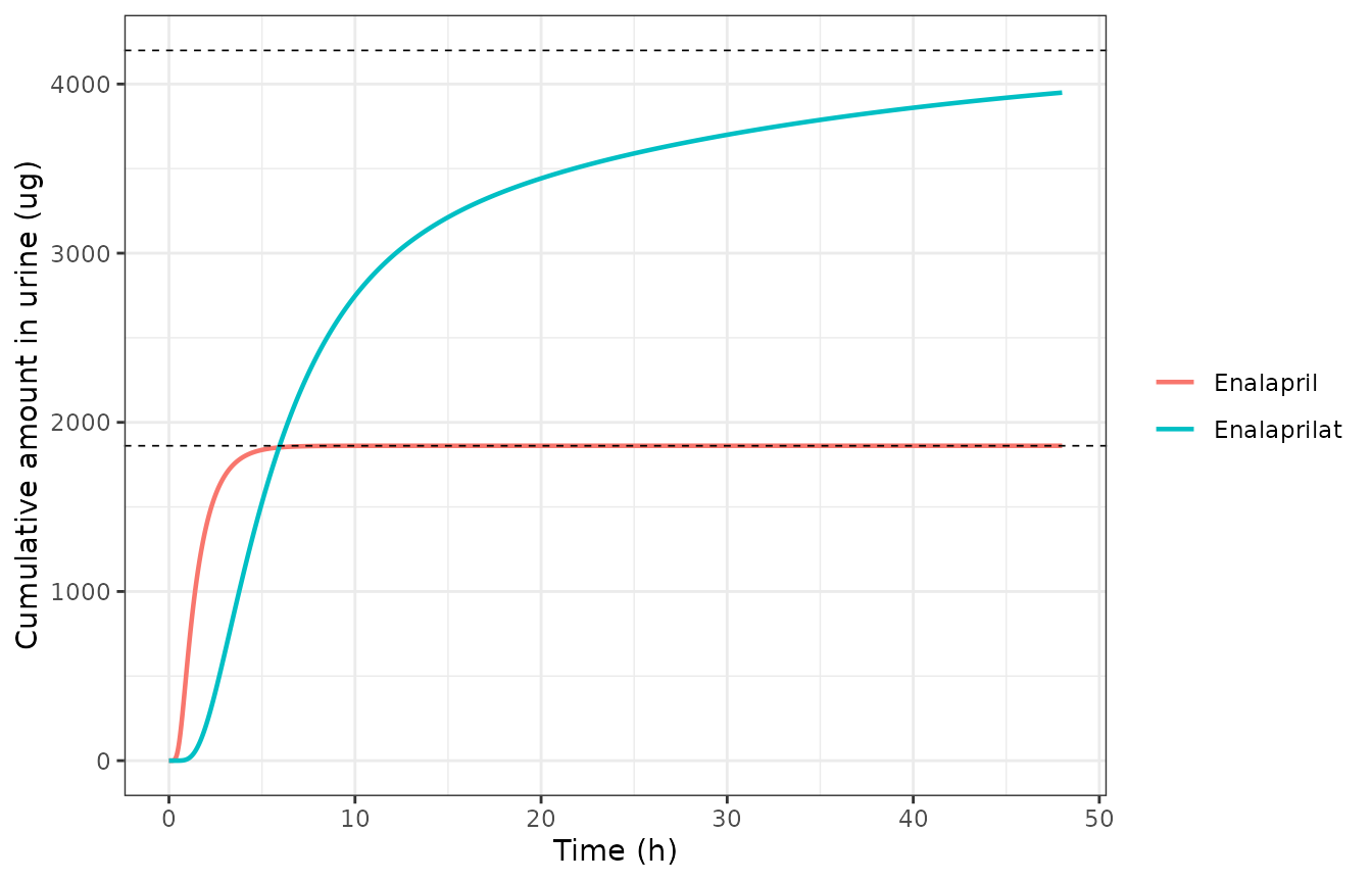

Typical-value cumulative urinary excretion of enalapril and enalaprilat over the trial’s 48 h collection window. Reproduces the median behaviour of the VPC panels B and D of Figure 3 of Faisal 2019; dashed lines are the closed-form asymptotes.

The formulation effect, three ways

The paper establishes its headline result twice over: once as a covariate in the pooled model, and once by comparing the two formulation-specific fits. Both are packaged, so both can be reproduced.

thetaOf <- function(nm) rxode2::rxode2(readModelDb(nm))$theta

mttPooledRef <- exp(thetaOf("Faisal_2019_enalapril")[["lmtt"]])
#> ℹ parameter labels from comments will be replaced by 'label()'
formEffect <- thetaOf("Faisal_2019_enalapril")[["e_form_odmt_mtt"]]
#> ℹ parameter labels from comments will be replaced by 'label()'
mttSepRef <- exp(thetaOf("Faisal_2019_enalapril_reference")[["lmtt"]])
#> ℹ parameter labels from comments will be replaced by 'label()'
mttSepOdmt <- exp(thetaOf("Faisal_2019_enalapril_odmt")[["lmtt"]])
#> ℹ parameter labels from comments will be replaced by 'label()'

data.frame(
  Analysis = c("Pooled model (Table 1, covariate)", "Separate fits (Tables Supp-I / Supp-II)"),
  `MTT1 reference (h)` = c(mttPooledRef, mttSepRef),
  `MTT1 ODMT (h)` = c(mttPooledRef * formEffect, mttSepOdmt),
  check.names = FALSE
) |>
  mutate(`Difference (min)` = 60 * (`MTT1 reference (h)` - `MTT1 ODMT (h)`)) |>
  knitr::kable(digits = c(0, 3, 3, 1))

Analysis	MTT1 reference (h)	MTT1 ODMT (h)	Difference (min)
Pooled model (Table 1, covariate)	0.558	0.407	9.0
Separate fits (Tables Supp-I / Supp-II)	0.570	0.484	5.2

# The paper's abstract, Results and Conclusion all state "5 min" for the
# separate-fit comparison; this is a fixed published number, not a draw.
stopifnot(
  abs(60 * (mttSepRef - mttSepOdmt) - 5) < 1,
  # The ODMT shortens MTT1 in the pooled model too (direction of theta_12).
  formEffect < 1
)

The separate fits give 5.2 min, matching the paper’s repeated “5 min” claim exactly. The pooled model’s covariate implies a larger 9.0 min shift; the two need not agree, because the pooled model forces the eight-transit chain on the ODMT arm whereas the ODMT-specific fit uses six, and a shorter chain reaches the same onset with a longer mean transit time. Both analyses agree on sign and on the qualitative conclusion, which is what the paper claims.

Virtual cohort and PKNCA

A stochastic cohort of 100 subjects per formulation arm, sampled at the trial’s own serum schedule. Body weights are drawn to match the Table 2 summary (mean 69.76 kg) and truncated to the observed 51.8-95.6 kg range; the paper does not publish the weight distribution’s shape, so a log-normal is assumed (see Errata).

rxode2::rxSetSeed(20190709)
set.seed(20190709)

nPerArm <- 100
serumTimes <- c(0, 0.17, 0.33, 0.5, 0.75, 1, 1.25, 1.5, 2, 2.5, 3, 3.5, 4,
                4.5, 5, 6, 8, 10, 12, 24, 48)

drawWt <- function(n) {
  w <- numeric(0)
  while (length(w) < n) {
    cand <- stats::rlnorm(2 * n, meanlog = log(69.76) - 0.5 * 0.16^2, sdlog = 0.16)
    w <- c(w, cand[cand >= 51.8 & cand <= 95.6])
  }
  w[seq_len(n)]
}

subj <- data.frame(
  id = seq_len(2 * nPerArm),
  FORM_ODMT = rep(c(0, 1), each = nPerArm),
  WT = c(drawWt(nPerArm), drawWt(nPerArm))
) |>
  mutate(treatment = if_else(FORM_ODMT == 1, "ODMT", "Reference tablet"))

doseRows <- subj |>
  transmute(id, time = 0, amt = doseUg, evid = 1L, cmt = "transit1")
obsRows <- tidyr::expand_grid(id = subj$id, time = serumTimes) |>
  transmute(id, time, amt = NA_real_, evid = 0L, cmt = "Cc")

events <- bind_rows(doseRows, obsRows) |>
  arrange(id, time, desc(evid)) |>
  left_join(select(subj, id, WT, FORM_ODMT), by = "id")

sim <- rxode2::rxSolve(mPooled, events, returnType = "data.frame", useLinCmt = FALSE) |>
  left_join(select(subj, id, treatment), by = "id")

nrow(sim)
#> [1] 4200

sim |>
  select(id, time, treatment, Enalapril = Cc, Enalaprilat = Cc_enaat) |>
  pivot_longer(c(Enalapril, Enalaprilat), names_to = "Analyte", values_to = "conc") |>
  filter(time <= 24) |>
  group_by(treatment, Analyte, time) |>
  summarise(
    lo = quantile(conc, 0.025), md = median(conc), hi = quantile(conc, 0.975),
    .groups = "drop"
  ) |>
  ggplot(aes(time, md, colour = treatment, fill = treatment)) +
  geom_ribbon(aes(ymin = lo, ymax = hi), alpha = 0.15, colour = NA) +
  geom_line(linewidth = 0.8) +
  facet_wrap(~Analyte, scales = "free_y") +
  labs(x = "Time (h)", y = "Serum concentration (ug/L)", colour = NULL, fill = NULL) +
  theme_bw()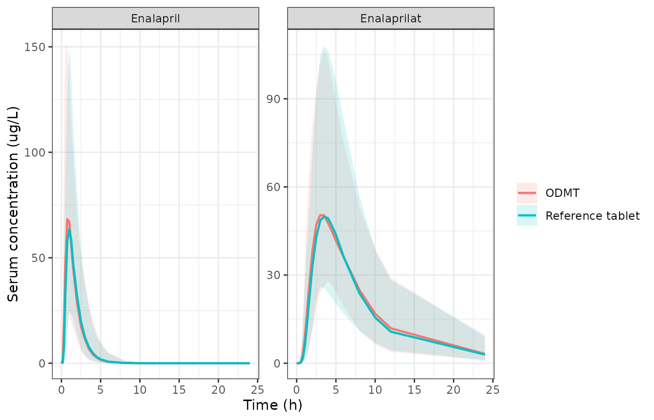

Simulated serum enalapril and enalaprilat concentrations (median and 2.5th-97.5th percentiles) by formulation. Compare Figure 3 panels A and C of Faisal 2019.

NCA is run with PKNCA, one block per serum analyte, grouped by treatment so per-formulation results can be compared.

Simulated profiles are noise-free and decay to arbitrarily small numbers, which real assay data do not. Left uncensored, PKNCA’s automatic lambda.z window selection reaches from 1.25 h – still on the absorption curve – out to 48 h at around 1e-14 ug/L, giving an adjusted r-squared of 0.95 and a terminal half-life biased ~40% high. Below-LLOQ records are therefore dropped before NCA, exactly as the trial did (“Study samples measured below the LLOQ were not included”), using the paper’s reported serum LLOQs of 0.195 ng/mL for enalapril and 0.180 ng/mL for enalaprilat. The time-zero record is always retained so that no AUC interval starts before the first measurement.

lloq <- c(Cc = 0.195, Cc_enaat = 0.180) # ug/L; Methods, "Bioanalysis of Serum and Urine Samples"

ncaFor <- function(concCol) {
  cdat <- sim |>
    transmute(id, treatment, time, conc = .data[[concCol]]) |>
    filter(!is.na(conc), time == 0 | conc >= lloq[[concCol]])
  ddat <- subj |> transmute(id, treatment, time = 0, dose = doseUg)
  # The concentration formula carries the treatment grouping so results can be
  # compared per formulation; PKNCAdose does not accept a nested (slash)
  # formula, so the dose side groups by subject only.
  o_conc <- PKNCA::PKNCAconc(cdat, conc ~ time | id / treatment)
  o_dose <- PKNCA::PKNCAdose(ddat, dose ~ time | id)
  PKNCA::pk.nca(PKNCA::PKNCAdata(
    o_conc, o_dose,
    intervals = data.frame(
      start = 0, end = Inf,
      cmax = TRUE, tmax = TRUE, auclast = TRUE, aucinf.obs = TRUE, half.life = TRUE
    )
  ))
}

ncaEna <- ncaFor("Cc")
ncaEnaat <- ncaFor("Cc_enaat")

bind_rows(
  as.data.frame(ncaEna$result) |> mutate(Analyte = "Enalapril"),
  as.data.frame(ncaEnaat$result) |> mutate(Analyte = "Enalaprilat")
) |>
  filter(PPTESTCD %in% c("cmax", "tmax", "auclast", "aucinf.obs", "half.life")) |>
  group_by(Analyte, treatment, PPTESTCD) |>
  summarise(Median = median(PPORRES, na.rm = TRUE), .groups = "drop") |>
  mutate(Parameter = nlmixr2lib::ncaParamLabel(PPTESTCD)) |>
  select(Analyte, treatment, Parameter, Median) |>
  pivot_wider(names_from = treatment, values_from = Median) |>
  knitr::kable(digits = 3)

Analyte	Parameter	ODMT	Reference tablet
Enalapril	AUC0-∞ (obs)	116.930	115.704
Enalapril	AUClast	116.594	114.831
Enalapril	Cmax	74.829	70.198
Enalapril	t½	0.714	0.714
Enalapril	Tmax	0.750	1.000
Enalaprilat	AUC0-∞ (obs)	467.714	471.853
Enalaprilat	AUClast	453.132	451.276
Enalaprilat	Cmax	50.957	52.583
Enalaprilat	t½	9.469	9.178
Enalaprilat	Tmax	3.500	3.500

Comparison against published values

Faisal 2019 publishes no NCA table, so there is no like-for-like Cmax/AUC reference to compare against. What it does publish, and what the companion individual-fit paper on the same trial publishes, are the quantities below. The enalapril half-life reference is derived from the companion paper’s reference-arm elimination rate constant KE = 1.143 1/h (Table 4, geometric mean), and the Tmax references are the main paper’s own Results prose.

simNca <- bind_rows(
  as.data.frame(ncaEna$result) |> mutate(Analyte = "Enalapril"),
  as.data.frame(ncaEnaat$result) |> mutate(Analyte = "Enalaprilat")
) |>
  filter(treatment == "Reference tablet", PPTESTCD %in% c("tmax", "half.life")) |>
  select(Analyte, PPTESTCD, PPORRES)

refNca <- data.frame(
  Analyte = c("Enalapril", "Enalaprilat"),
  tmax = c(1.0, 3.5),
  half.life = c(log(2) / 1.143, NA_real_)
)

cmp <- nlmixr2lib::ncaComparisonTable(
  simNca, refNca,
  by = "Analyte",
  units = c(tmax = "h", half.life = "h"),
  tolerance_pct = 20
)
knitr::kable(cmp, digits = 3)

NCA parameter	Analyte	Reference	Simulated	% diff
Tmax (h)	Enalapril	1	1	+0.0%
Tmax (h)	Enalaprilat	3.5	3.5	+0.0%
t½ (h)	Enalapril	0.606	0.714	+17.8%
t½ (h)	Enalaprilat	—	9.18	—

attr(cmp, "footnote")
#> NULL

Two further published quantities are checked directly rather than through the NCA table.

th <- thetaOf("Faisal_2019_enalapril")
#> ℹ parameter labels from comments will be replaced by 'label()'
ktot <- exp(th[["lkurine"]]) + exp(th[["lkmet"]])
vcOverF <- exp(th[["lvc"]]) / exp(th[["lfdepot"]])

data.frame(
  Quantity = c(
    "Total enalapril elimination rate constant (1/h)",
    "Apparent enalapril volume VC/F1 (L)"
  ),
  Published = c(0.94, NA),
  `This model` = c(ktot, vcOverF),
  Source = c(
    "Weisser 1991 via Faisal 2019 Discussion (0.94 1/h)",
    "companion paper Table 4 VD/f: 69.7, 72.5, 80.5 L across the three arms"
  ),
  check.names = FALSE
) |>
  knitr::kable(digits = 3)

Quantity	Published	This model	Source
Total enalapril elimination rate constant (1/h)	0.94	0.993	Weisser 1991 via Faisal 2019 Discussion (0.94 1/h)
Apparent enalapril volume VC/F1 (L)	NA	84.323	companion paper Table 4 VD/f: 69.7, 72.5, 80.5 L across the three arms

# Published point values, not cohort draws -> exact bounds are appropriate.
stopifnot(
  # Faisal 2019 Discussion cross-checks the summed elimination rate against
  # the literature value of 0.94 1/h.
  abs(ktot - 0.94) / 0.94 < 0.10,
  # The apparent volume must land in the neighbourhood of the companion
  # paper's individual-fit VD/f range (69.7-80.5 L across three arms).
  vcOverF > 60, vcOverF < 105
)

The summed elimination rate constant is 0.993 1/h against the literature’s 0.94 1/h, and VC/F1 is 84.3 L against the companion paper’s 69.7-80.5 L from a structurally different (one-compartment, lag-time) individual fit on the same subjects. Both agree to within the difference the two model structures would be expected to produce.

No row in the NCA comparison exceeds the 20% flagging tolerance. The largest residual difference is the enalapril terminal half-life, 0.714 h simulated against 0.606 h implied by the companion paper’s KE. That gap is a genuine between-model difference rather than an implementation error: the simulated value recovers this model’s own structural half-life, ln(2) / (KREN + KM) = ln(2) / 0.993 = 0.698 h, to within 2%, and the companion paper reaches a faster KE because it attributes the whole absorption delay to a lag time and a single first-order KA, whereas Faisal 2019 spreads it across an eight-compartment transit chain. The two papers fit the same subjects with different absorption structures, so their terminal-phase estimates are not expected to coincide exactly.

Assumptions and deviations

THETA (X) is read as the formulation effect theta_12, not the weight exponent. Table 1’s final structural row is labelled only THETA (X) = 0.730 (12.0% RSE), yet the final model carries two covariate effects (weight on VC, formulation on MTT1) and the table has room for only one coefficient. Three independent lines of evidence resolve this in favour of theta_12:

The Methods state that for the weight relationship “the parameter theta was tested with a fixed value of 1 for the volume of distribution and 0.75 for clearance.” Weight was retained only on VC, a volume. A parameter fixed at 1 has no standard error and would not appear in a parameter table; the tabulated 0.730 carries a 12.0% RSE, so it was estimated.
The label THETA (X) matches the notation family of Equation 7 (TV = theta_X * theta_12^FORM * exp(eta)), not the bare theta exponent of Equation 6.
The row is absent from both Supplementary Tables Supp-I and Supp-II, which are single-formulation fits and therefore cannot carry a formulation effect – but which would still need a weight exponent if one had been estimated.

The model file therefore encodes e_wt_vc <- fixed(1) and e_form_odmt_mtt <- 0.730. No value is invented under this reading; the alternative reading would leave theta_12 unreported and require one.

Dose basis: labelled enalapril maleate, not free base. Neither Faisal 2019 nor its companion states whether the modelled AMT was the labelled 10 mg of enalapril maleate or the equivalent 7.643 mg of enalapril free base (molecular weights 492.52 and 376.45; ratio 0.76433). The maleate reading is used here, because (a) the paper benchmarks its estimated F1 = 0.606 against a literature figure of “60% of drug absorption”, which is conventionally expressed as a fraction of the administered, labelled dose, and (b) the companion paper describes the dose as “10 mg” throughout with no salt correction and reports VD/f of 69.7-80.5 L, which brackets this model’s VC/F1 = 84.3 L under the maleate reading but not under the free-base reading (64.4 L). This differs from Steichert_2025_enalapril_enalaprilat_pediatric, which requires free base; multiply or divide by 0.76433 to move a dose between the two models.

The weight covariate is carried into the two formulation-specific models. Supplementary Tables Supp-I and Supp-II report no covariate coefficient, but both are headed “FINAL (FULL) MODEL” – the same label Table 1 uses for the covariate-carrying pooled model – and an exponent fixed at 1 produces no table row. The weight term is therefore included in all three model files. Because the exponent is fixed at 1, this is the identity at the reference weight and the choice is consequential only away from 69.76 kg.

MTT = (N + 1) / KTR with a separately estimated KA. This is an unusual combination – Savic’s (n + 1) convention normally absorbs the final transfer into KTR – but the paper prints it that way in both the Methods text and the Figure 1 annotation while also estimating KA as a distinct parameter, and the printed equation is followed as written.

Internal inconsistencies in the source (errata). The Discussion quotes several values that do not match Table 1: the summed elimination rate constant as “0.93 1/h” (Table 1 implies 0.305 + 0.688 = 0.993), the enalaprilat elimination rate constant as “0.175 1/h” (Table 1 gives 0.184; 0.175 is the ODMT-only value from Supplementary Table Supp-II), and KA as “6.03 1/h” against Table 1’s 6.010. The parameter tables are treated as authoritative throughout. Table 1’s bootstrap CI for KQ2 is printed as “0.048-0.620”, which is almost certainly a typo for 0.062 given the SIR interval of 0.046-0.063; CIs are not carried into the model file, so nothing depends on it.

Residual-error scale. Table 1 labels the proportional rows “Proportional error (sigma 2)” and the additive rows “Additive error (ug/l)”. The proportional values are therefore variances and are entered as sqrt(), while the additive values are already on the SD scale. The resulting proportional CV of 10% for serum enalapril is consistent with the reported assay intermediate precision of 5.0-9.5%, and the additive SDs of 0.188 and 0.220 ug/L sit at the reported serum LLOQs of 0.195 and 0.180 ng/mL – both of which are what these quantities should look like, and neither of which would hold under the opposite reading.

Not modelled. Age, height, sex and total body water were available as candidate covariates (Table 2) and screened, but only weight was retained, so they are recorded in the population metadata rather than as covariateData entries. The paper reports no IIV on KQ1 or KQ2 and none is invented. No inter-occasion variability was estimated despite the crossover design.

Below-LLOQ censoring before NCA. Simulated concentrations are noise-free and continue decaying long past anything an assay could measure. Feeding them to PKNCA uncensored lets the automatic lambda.z window start at 1.25 h – still inside the absorption phase – and run to 48 h at ~1e-14 ug/L, which biases the enalapril terminal half-life to 0.99 h (adjusted r-squared 0.95) against a structural value of 0.698 h. Post-dose records below the paper’s reported serum LLOQs (0.195 ng/mL enalapril, 0.180 ng/mL enalaprilat) are therefore dropped before NCA, which is what the trial itself did. This is a property of simulated data, not a parameter adjustment: no model value is changed, and the censored NCA recovers the model’s own structural half-life to within 2%.

Simulation assumptions. The virtual cohort’s weight distribution is assumed log-normal with the published mean and truncated to the published range; the paper reports only mean, median, minimum and maximum. Sex and age are not simulated because they enter no model parameter. The cohort is 100 subjects per arm, which is ample for the median-and-interval summaries shown and well inside the library’s 200-per-arm cap.