Cefpirome (Bulitta 2011)
Source:vignettes/articles/Bulitta_2011_cefpirome.Rmd
Bulitta_2011_cefpirome.RmdModel and source
- Citation: Bulitta JB, Kinzig M, Landersdorfer CB, Holzgrabe U, Stephan U, Sorgel F. Comparable Population Pharmacokinetics and Pharmacodynamic Breakpoints of Cefpirome in Cystic Fibrosis Patients and Healthy Volunteers. Antimicrob Agents Chemother. 2011 Jun;55(6):2927-2936. doi:10.1128/AAC.01484-10
- Description: Three-compartment population PK model for IV cefpirome with simultaneous fit of plasma concentrations and amounts excreted unchanged in urine. Built from a pooled cohort of 24 Caucasian adults: 12 cystic fibrosis (CF) patients and 12 healthy volunteers (HVs) each given a single 10-min IV infusion of 2 g cefpirome. Body size is captured by allometric scaling on lean body mass (LBM) with fixed exponents 0.75 on clearance terms and 1.0 on volumes (reference LBM = 53 kg). Total clearance is split into an estimated renal arm (CL_R, urinary recovery is tracked in the canonical urine compartment) and a non-renal arm (CL_NR). A CF / HV cohort indicator DIS_CF (1 = CF patient, 0 = HV reference) carries three disease- specific scale factors estimated by the paper: FCYF_CLR = 1.07 applied to CL_R, FCYF_CLNR = 1.13 applied to CL_NR, and FCYF_VSS = 0.98 applied uniformly to V1 (central), V2 (shallow peripheral), and V3 (deep peripheral). The inter-compartmental clearances Q12 (central <-> shallow) and Q23 (central <-> deep) are shared across cohorts. Typical-value clearance and volume estimates are anchored to DIS_CF = 0 (HV reference) per the DIS_CF covariate convention registered in inst/references/covariate-columns.md.
- Article: https://doi.org/10.1128/AAC.01484-10
Population
Bulitta 2011 fit a unified three-compartment population PK model to pooled data from 24 Caucasian adults (paper Table 1):
- 12 adult cystic-fibrosis (CF) patients: total body weight 31.5-66.5 kg (median 53.3), lean body mass 26.2-55.9 kg (median 45.7), age 18-34 years (median 22.5), 8 male / 4 female, all with normal renal function (estimated creatinine clearance 89.3-164 mL/min, median 131).
- 12 matched adult healthy volunteers (HVs): total body weight 53.0-85.0 kg (median 63.6), lean body mass 41.8-62.7 kg (median 50.0), age 20-35 years (median 29), 6 male / 6 female, estimated creatinine clearance 92.3-150 mL/min (median 116).
Each subject received a single 10-min IV infusion of 2 g cefpirome
dissolved in 20 mL water for injection. Plasma samples were drawn at 5
min and 10 min after the start of infusion and at 5, 10, 15, 20, 30 min
and 0.75, 1, 1.25, 1.5, 2, 2.5, 3, 4, 5, 6, 7, 8, 10, 12, 16, and 24 h
after the end of infusion. Urine was collected from the start of the
infusion to 1 h after end of infusion and then in 10 intervals out to 48
h. Population PK estimation used NONMEM VI level 1.2 with
FOCE+INTERACTION and a parallel S-ADAPT MC-PEM analysis; the NONMEM
estimates were used for the Monte Carlo simulations and are encoded in
the nlmixr2lib model file. The same demographic information is available
programmatically via
readModelDb("Bulitta_2011_cefpirome")$population.
Source trace
The per-parameter origin is recorded as an in-file comment next to
each ini() entry in
inst/modeldb/specificDrugs/Bulitta_2011_cefpirome.R. The
table below collects them in one place for review.
| Equation / parameter | Value | Source location |
|---|---|---|
lcl_renal |
log(5.78) | Table 3 NONMEM HV column (CL_R) |
lcl_nonren |
log(1.17) | Table 3 NONMEM HV column (CL_NR) |
lvc |
log(7.44) | Table 3 NONMEM HV column (V1) |
lvp |
log(2.67) | Table 3 NONMEM HV column (V2) |
lvp2 |
log(4.63) | Table 3 NONMEM HV column (V3) |
lq |
log(25.6) | Table 3 NONMEM (CLic_shallow; single value) |
lq2 |
log(2.81) | Table 3 NONMEM (CLic_deep; single value) |
e_lbm_cl_q |
fixed(0.75) | Population PK / Body size paragraph |
e_lbm_vc_vp |
fixed(1.00) | Population PK / Body size paragraph |
e_cf_cl_renal |
log(1.07) = +0.06766 | Table 4 LBM-allometric row (FCYF_CLR) |
e_cf_cl_nonren |
log(1.13) = +0.12222 | Table 4 LBM-allometric row (FCYF_CLNR) |
e_cf_vc_vp_vp2 |
log(0.98) = -0.02020 | Table 4 LBM-allometric row (FCYF_VSS) |
etalcl_renal |
0.135^2 = 0.018225 | Table 3 NONMEM BSV(CL_R), apparent CV |
etalcl_nonren |
0.322^2 = 0.103684 | Table 3 NONMEM BSV(CL_NR), apparent CV |
etalvc (block diagonal) |
0.448^2 = 0.200704 | Table 3 NONMEM BSV(V1), apparent CV |
etalvp (block diagonal) |
0.735^2 = 0.540225 | Table 3 NONMEM BSV(V2), apparent CV |
cov(etalvc, etalvp) |
-0.838 * 0.448 * 0.735 = -0.275893 | Table 3 footnote d (r(V1,V2) = -0.838) |
etalvp2 |
0.111^2 = 0.012321 | Table 3 NONMEM BSV(V3), apparent CV |
| BSV on q, q2 | not estimated | Table 3 NONMEM: BSV(CLic_shallow/_deep) = 0 fix |
propSd, addSd |
0.0875, 0.429 | Table 3 NONMEM (CV_C, SD_C, plasma) |
propSd_urineAmt, addSd_urineAmt |
0.182, 6.12 | Table 3 NONMEM (CV_AU, SD_AU, urine) |
| Three-compartment ODE structure | n/a | Methods (Population PK analysis, Population model paragraph) |
| Urinary excretion compartment | n/a | Methods (simultaneous fitting plasma + urine) |
| DIS_CF cohort encoding | n/a | Methods (Population PK / BSV model paragraph: FCYF scale factors) |
Virtual cohort
Original observed data are not publicly available. The simulation below uses a virtual population of 200 CF patients and 200 healthy volunteers whose lean body mass distributions approximate the cohort medians and ranges reported in Bulitta 2011 Table 1.
set.seed(20110614)

make_cohort <- function(n, lbm_mu, lbm_sd, lbm_min, lbm_max, dis_cf, label, id_offset) {
  tibble(
    id     = id_offset + seq_len(n),
    LBM    = pmin(pmax(rnorm(n, mean = lbm_mu, sd = lbm_sd), lbm_min), lbm_max),
    DIS_CF = dis_cf,
    cohort = label
  )
}

n_per_cohort <- 200L

cohort_cf <- make_cohort(
  n        = n_per_cohort,
  lbm_mu   = 45.7,
  lbm_sd   = 8.0,
  lbm_min  = 26.2,
  lbm_max  = 55.9,
  dis_cf   = 1L,
  label    = "CF patient",
  id_offset = 0L
)

cohort_hv <- make_cohort(
  n        = n_per_cohort,
  lbm_mu   = 50.0,
  lbm_sd   = 6.0,
  lbm_min  = 41.8,
  lbm_max  = 62.7,
  dis_cf   = 0L,
  label    = "Healthy volunteer",
  id_offset = n_per_cohort
)

cohorts <- bind_rows(cohort_cf, cohort_hv)
Each subject receives a single 2 g IV infusion administered over 10 minutes, matching the dosing scheme described in paper Methods (Study design and drug administration paragraph).
infusion_dur_h <- 10 / 60   # 10-min infusion expressed in hours
dose_amt_mg    <- 2000

obs_times <- c(
  seq(0,  0.25, by = 0.025),     # dense around end-of-infusion
  seq(0.5, 4,   by = 0.25),      # alpha/beta phase
  seq(4.5, 24,  by = 0.5)        # terminal sampling out to 24 h
)

dose_rows <- cohorts |>
  mutate(
    time = 0,
    evid = 1L,
    amt  = dose_amt_mg,
    cmt  = "central",
    rate = dose_amt_mg / infusion_dur_h,
    dv   = NA_real_
  )

obs_rows <- cohorts |>
  tidyr::crossing(time = obs_times) |>
  mutate(
    evid = 0L,
    amt  = NA_real_,
    cmt  = "Cc",
    rate = 0,
    dv   = NA_real_
  )

# Cumulative-urine observations at the end of each collection interval
# (matched to paper Methods: 1, 2, 3, 4, 6, 8, 10, 12, 24, 36, 48 h truncated
# to the 24-h window covered by the plasma simulation).
urine_times <- c(1, 2, 3, 4, 6, 8, 10, 12, 24)

urine_rows <- cohorts |>
  tidyr::crossing(time = urine_times) |>
  mutate(
    evid = 0L,
    amt  = NA_real_,
    cmt  = "urineAmt",
    rate = 0,
    dv   = NA_real_
  )

events <- bind_rows(dose_rows, obs_rows, urine_rows) |>
  arrange(id, time, desc(evid))

stopifnot(!anyDuplicated(unique(events[, c("id", "time", "evid", "cmt")])))
Simulation
mod <- readModelDb("Bulitta_2011_cefpirome")

sim <- rxode2::rxSolve(
  mod,
  events = events,
  keep   = c("cohort", "LBM", "DIS_CF")
) |>
  as.data.frame()
#> ℹ parameter labels from comments will be replaced by 'label()'

# When multiple endpoints (Cc and urineAmt) are observed at the same time, the
# simulation returns one row per CMT channel. The `Cc` and `urineAmt` columns
# are populated identically at coincident times, so distinct (id, time) rows
# are enough for the per-output figures and the NCA step.
sim_unique <- sim |>
  dplyr::distinct(id, time, .keep_all = TRUE)
Replicate published figures
The simulated population recapitulates the cohort-stratified visual predictive check shown in Bulitta 2011 Figure 1: CF patients and healthy volunteers exhibit superimposable plasma concentration-time profiles after a 2 g IV infusion administered to subjects of similar lean body mass, with CF patients showing a marginal terminal-phase shift consistent with their 20% higher total clearance per kilogram of total body weight (paper Discussion).
sim_unique |>
  dplyr::filter(!is.na(Cc), Cc > 0) |>
  dplyr::group_by(cohort, time) |>
  dplyr::summarise(
    Q05 = quantile(Cc, 0.05, na.rm = TRUE),
    Q50 = quantile(Cc, 0.50, na.rm = TRUE),
    Q95 = quantile(Cc, 0.95, na.rm = TRUE),
    .groups = "drop"
  ) |>
  ggplot(aes(time, Q50, fill = cohort, colour = cohort)) +
  geom_ribbon(aes(ymin = Q05, ymax = Q95), alpha = 0.25, colour = NA) +
  geom_line(linewidth = 0.7) +
  scale_y_log10() +
  labs(
    x = "Time after start of infusion (h)",
    y = "Cefpirome plasma concentration (mg/L)",
    fill   = NULL,
    colour = NULL,
    title  = "Plasma concentration-time profile after 2 g IV (median + 90% PI)",
    caption = "Approximates the VPC structure of Bulitta 2011 Figure 1 (top)."
  ) +
  theme_minimal()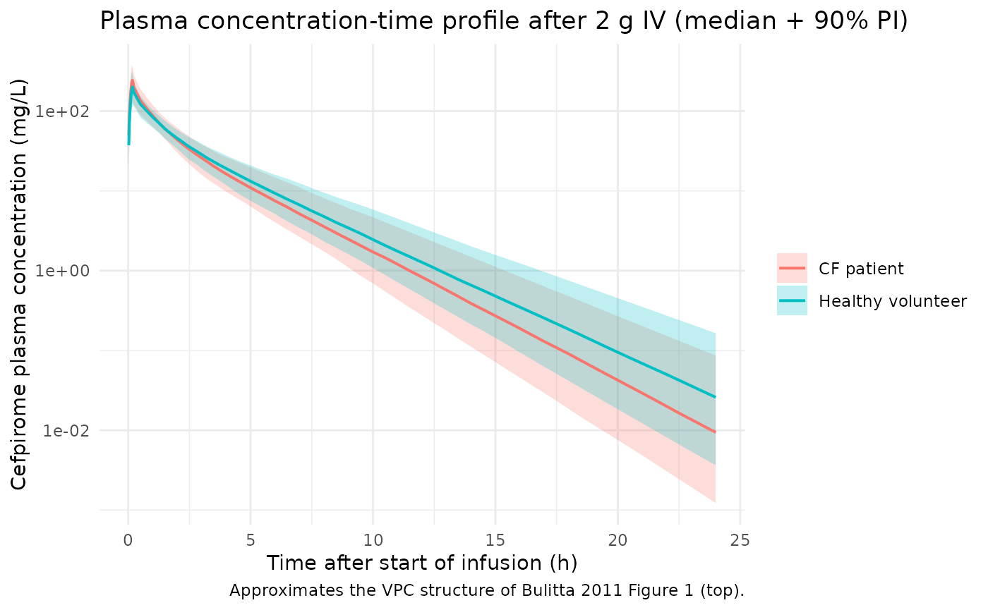
sim_unique |>
  dplyr::filter(!is.na(urineAmt)) |>
  dplyr::group_by(cohort, time) |>
  dplyr::summarise(
    Q05 = quantile(urineAmt, 0.05, na.rm = TRUE),
    Q50 = quantile(urineAmt, 0.50, na.rm = TRUE),
    Q95 = quantile(urineAmt, 0.95, na.rm = TRUE),
    .groups = "drop"
  ) |>
  ggplot(aes(time, Q50, fill = cohort, colour = cohort)) +
  geom_ribbon(aes(ymin = Q05, ymax = Q95), alpha = 0.25, colour = NA) +
  geom_line(linewidth = 0.7) +
  labs(
    x = "Time after start of infusion (h)",
    y = "Cumulative cefpirome amount in urine (mg)",
    fill   = NULL,
    colour = NULL,
    title  = "Cumulative urinary excretion after 2 g IV (median + 90% PI)",
    caption = "Approximates the VPC structure of Bulitta 2011 Figure 1 (middle)."
  ) +
  theme_minimal()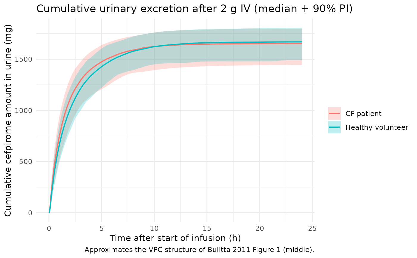
PKNCA validation
We compute NCA parameters on the simulated plasma concentration
profile following the single 2 g IV infusion using PKNCA. The treatment
grouping (cohort) allows the simulated Cmax, AUC, and
terminal half-life to be compared against the cohort-stratified observed
values in paper Table 2.
sim_nca <- sim_unique |>
  dplyr::filter(!is.na(Cc), Cc > 0) |>
  dplyr::select(id, time, Cc, cohort)

conc_obj <- PKNCA::PKNCAconc(
  sim_nca, Cc ~ time | cohort + id,
  concu = "mg/L", timeu = "h"
)

dose_df <- cohorts |>
  dplyr::mutate(time = 0, amt = dose_amt_mg)

dose_obj <- PKNCA::PKNCAdose(
  dose_df, amt ~ time | cohort + id,
  doseu = "mg"
)

intervals <- data.frame(
  start       = 0,
  end         = Inf,
  cmax        = TRUE,
  tmax        = TRUE,
  aucinf.obs  = TRUE,
  half.life   = TRUE,
  cl.obs      = TRUE
)

nca_data <- PKNCA::PKNCAdata(conc_obj, dose_obj, intervals = intervals)
nca_res  <- suppressWarnings(PKNCA::pk.nca(nca_data))

nca_long <- as.data.frame(nca_res$result) |>
  dplyr::filter(PPTESTCD %in% c("cmax", "tmax", "aucinf.obs", "half.life", "cl.obs"))

nca_summary <- nca_long |>
  dplyr::group_by(cohort, PPTESTCD) |>
  dplyr::summarise(
    median = stats::median(PPORRES, na.rm = TRUE),
    q05    = stats::quantile(PPORRES, 0.05, na.rm = TRUE),
    q95    = stats::quantile(PPORRES, 0.95, na.rm = TRUE),
    .groups = "drop"
  ) |>
  dplyr::mutate(
    formatted = sprintf("%.2f (%.2f-%.2f)", median, q05, q95)
  ) |>
  dplyr::select(cohort, PPTESTCD, formatted) |>
  tidyr::pivot_wider(names_from = PPTESTCD, values_from = formatted)

knitr::kable(
  nca_summary,
  caption = "Simulated noncompartmental parameters (median, 5%-95% prediction interval) by cohort."
)| cohort | aucinf.obs | cl.obs | cmax | half.life | tmax |
|---|---|---|---|---|---|
| CF patient | NA (NA-NA) | NA (NA-NA) | 242.92 (129.22-373.24) | 1.86 (1.51-2.50) | 0.18 (0.15-0.18) |
| Healthy volunteer | NA (NA-NA) | NA (NA-NA) | 201.05 (120.07-313.25) | 2.12 (1.70-2.73) | 0.18 (0.15-0.18) |
Cumulative urinary fraction excreted unchanged at 24 h
urine_recovery <- sim_unique |>
  dplyr::filter(!is.na(urineAmt), time == 24) |>
  dplyr::mutate(fer = urineAmt / dose_amt_mg) |>
  dplyr::group_by(cohort) |>
  dplyr::summarise(
    median = stats::median(fer, na.rm = TRUE),
    q05    = stats::quantile(fer, 0.05, na.rm = TRUE),
    q95    = stats::quantile(fer, 0.95, na.rm = TRUE),
    .groups = "drop"
  ) |>
  dplyr::mutate(
    formatted = sprintf("%.3f (%.3f-%.3f)", median, q05, q95)
  ) |>
  dplyr::select(cohort, formatted)

urine_recovery |>
  dplyr::rename(
    "Cohort"                            = cohort,
    "Fraction excreted unchanged (24 h)" = formatted
  ) |>
  knitr::kable(
    caption = "Simulated fraction excreted unchanged in urine at 24 h (median, 5%-95% PI) by cohort."
)| Cohort | Fraction excreted unchanged (24 h) |
|---|---|
| CF patient | 0.826 (0.721-0.899) |
| Healthy volunteer | 0.835 (0.745-0.903) |
Comparison against published NCA (Bulitta 2011 Table 2)
Paper Table 2 reports unscaled noncompartmental PK parameters for the 12 CF patients and the 12 healthy volunteers as median (minimum-maximum). The simulated values above target the same noncompartmental endpoints; the simulated Cmax depends on how densely the time grid is sampled around the end-of-infusion peak.
| Parameter | CF patients (observed) | Healthy volunteers (observed) |
|---|---|---|
| Total clearance (L/h) | 6.52 (4.05-8.51) | 6.64 (5.63-7.64) |
| Renal clearance (L/h) | 5.59 (3.18-9.98) | 5.51 (2.70-7.13) |
| Volume of distribution at steady state (L) | 14.4 (7.32-25.3) | 15.3 (12.6-19.4) |
| Fraction excreted unchanged (%) | 84.4 (78.6-100) | 87.0 (38.7-93.3) |
| Peak concentration (mg/L) | 221 (135-560) | 206 (159-299) |
| Terminal half-life (h) | 2.07 (1.95-3.29) | 2.17 (1.68-3.75) |
| Mean residence time (h) | 2.16 (1.58-3.03) | 2.33 (1.85-2.98) |
Differences of more than 20% between the simulated and observed columns typically indicate a transcription error in the source-trace; investigate the model file rather than tuning parameters. Note that paper Table 2 is the noncompartmental analysis of the observed data (linear scaling by total body weight, not allometric scaling by lean body mass), while the model in this package is the structural population PK model (LBM-allometric) underlying the Monte Carlo simulations in Bulitta 2011 Figure 2 and Table 6; minor discrepancies between Table 2 (noncompartmental) and Table 3 (population PK) typicals are expected.
Assumptions and deviations
-
DIS_CF encoding. The paper does not assign an
explicit covariate column name to the CF / healthy-volunteer cohort
flag; the CF-vs-HV split is encoded in the structural NONMEM / S-ADAPT
model via three group-scale factors FCYF_CLR, FCYF_CLNR, and FCYF_VSS
that multiply HV typical values for CF subjects. The model file encodes
the cohort flag as the new canonical binary covariate
DIS_CF(1 = CF patient, 0 = HV reference) registered ininst/references/covariate-columns.mdalongside this extraction. Typical values are anchored to the HV column of paper Table 3 so the published FCYF values are recovered as positive log-scale effects under theexp(e_cf_<param> * DIS_CF)form. -
FCYF_VSS applied uniformly to V1, V2, V3. The paper
estimates a single scale factor for volume of distribution at steady
state (FCYF_VSS), and the Table 3 V1, V2, V3 ratios CF/HV (0.976, 0.978,
0.976) are numerically indistinguishable from 0.98, consistent with a
single shared scale factor. The model file declares this as a single
shared covariate effect
e_cf_vc_vp_vp2applied uniformly to vc, vp, and vp2 inmodel(), extending the existing two-volume shared-exponent patterne_<cov>_vc_vp(perparameter-names.md) to the three-volume case. -
Inter-compartmental CL BSVs fixed at 0. Bulitta
2011 Table 3 reports BSV(CLic_shallow) and BSV(CLic_deep) as
0 (fixed)for the NONMEM analysis and0.15 (fixed)for the S-ADAPT analysis; the paper used the NONMEM estimates for the Monte Carlo simulations, soetalqandetalq2are omitted fromini(). Users running S-ADAPT-style simulations may add~ fixed(0.15^2)terms manually. -
Apparent-CV interpretation of BSV. Table 3 footnote
c labels the BSV values as “apparent coefficients of variation”,
interpreted as sqrt(omega^2) on the log scale; the back-transform used
here is omega^2 = (CV)^2 (not log(1 + CV^2)), matching the convention
used in
Jonckheere_2019_cefepime.Rand the broader Bulitta lab’s publications. -
V1-V2 correlation = -0.838. The paper retains only
the V1-V2 off-diagonal in the random-effect covariance matrix (footnote
d: “only the correlation of random effects in comparisons of V1 and V2
was included in the final model”); all other r^2 values were below 0.25
and not statistically significant. The model file encodes the block as
etalvc + etalvp ~ c(0.200704, -0.275893, 0.540225). - Cmax sampling density. The published Cmax estimates in paper Table 2 reflect a fixed sampling schedule that includes a sample at end of infusion (10 min). The simulated NCA Cmax in the vignette depends on the sampling density around end-of-infusion; if the user’s grid is coarser than the simulated grid here (0.025 h between 0 and 0.25 h), the simulated Cmax will fall below the published value because the end-of-infusion peak is the dominant feature.
-
10-min infusion duration. The model file declares
TK0 = 10 min as a fixed structural duration in the population
description and notes; users must supply the dosing infusion in the
event table via
rate = amt / (10/60)ordur = 10/60. The vignette simulates exactly this schedule. - Monte Carlo / breakpoint analysis out of scope. The paper’s Table 6 pharmacodynamic breakpoints (fT > MIC > 65%) were derived from 10,800- subject MCS at multiple dosing regimens. The vignette focuses on the structural PK validation; the breakpoint analysis is left as an exercise for users running site-specific MCS with the packaged model.