Reboxetine enantiomer binding kinetics at hNET (Benson 2010)
Source:vignettes/articles/Benson_2010_reboxetine_hnet_binding.Rmd
Benson_2010_reboxetine_hnet_binding.RmdModel and source
Benson 2010 measures how fast the two enantiomers of the antidepressant reboxetine bind to, and let go of, the human noradrenaline transporter (hNET). The experiment is a competition assay: a radiolabelled tracer, [3H]-desmethylimipramine (DMI), and an unlabelled competitor race for the same receptor pool, and only the tracer is counted. All three experiments (tracer saturation, tracer association, and drug-versus-tracer competition) were fit simultaneously in one NONMEM VI run, with each experiment treated as the “individual” of the mixed-effects model.
The paper presents two ODE systems and this package ships both.
mod_qsp <- rxode2::rxode(readModelDb("Benson_2010_reboxetine_qsp"))
#> ℹ parameter labels from comments will be replaced by 'label()'
mod_app <- rxode2::rxode(readModelDb("Benson_2010_reboxetine_apparent_qsp"))
#> ℹ parameter labels from comments will be replaced by 'label()'- Article: https://doi.org/10.1111/j.1476-5381.2010.00719.x (PMCID PMC2874860)
- Citation: Benson N, Snelder N, Ploeger B, Napier C, Sale H, Birdsall NJM, Butt RP, van der Graaf PH (2010). Estimation of binding rate constants using a simultaneous mixed-effects method: application to monoamine transporter reuptake inhibitor reboxetine. British Journal of Pharmacology 160(2):389-398. doi:10.1111/j.1476-5381.2010.00719.x. PMCID PMC2874860. Structural equations: Scheme 2 and Equations 10-15 (Methods, Mutually exclusive binding of enantiomers). Parameter values: Table 1 (mixed-effects analysis column) and the Results paragraph reporting Bmax.
| Model | Paper structure | What it is for |
|---|---|---|
Benson_2010_reboxetine_qsp |
Scheme 2, Equations 10-15 | Mechanistic. Tracer + SS-reboxetine + RR-reboxetine compete for hNET with enantiomer-specific rate constants. Setting one enantiomer to zero recovers the single-competitor Scheme 1 fit for the other. |
Benson_2010_reboxetine_apparent_qsp |
Scheme 1, Equations 1-5 | Phenomenological. Racemic reboxetine is fit as if it were one
ligand, giving the apparent koff,obs and
Kd,obs of Table 1. |
The split follows the paper. Benson 2010’s Discussion is explicit that the racemate is not a single molecular species and that “the parameter estimates [for] the racemate should be regarded as observed and not as molecularly defined properties”, so the two parameterisations are kept in separate files rather than merged.
Biological context
pop <- mod_qsp$population
tibble::tibble(Field = names(pop), Value = vapply(pop, \(x) paste(as.character(x), collapse = "; "), character(1))) |>
  dplyr::filter(Value != "NA") |>
knitr::kable(caption = "Population metadata (Benson 2010 Methods and Results).")| Field | Value |
|---|---|
| species | in vitro (HEK-293 cell membrane homogenate expressing recombinant human noradrenaline transporter, hNET; assay buffer 20 mM HEPES, 120 mM NaCl, 5 mM KCl, pH 7.4, room temperature ~25 C) |
| n_subjects | 53 |
| n_studies | 1 |
| race_ethnicity | |
| disease_state | In vitro radioligand binding assay; not a clinical population. |
| dose_range | Experiment 3 (competition kinetics, the source of the reboxetine estimates): unlabelled competitor at 0.1, 0.3 and 1 nM for racemic reboxetine and SS-reboxetine, and 1, 3, 10 and 30 nM for RR-reboxetine, against [3H]-DMI tracer at c. 1 nM and hNET at c. 0.1 nM. Experiment 1 (tracer saturation): [3H]-DMI 30 pM to 20 nM against c. 0.5 nM hNET. Experiment 2 (tracer association): [3H]-DMI typically 1.5 nM against c. 0.1 nM hNET. [3H]-SS-reboxetine saturation: 0.004 to 16 nM against c. 0.12 nM hNET. |
| notes | The mixed-effects ‘individual’ is an EXPERIMENT, not a subject: all data from Experiments 1-3 were analysed in a single NONMEM VI FOCE-I step over 1500 data points from 53 experiments (Benson 2010 Results). Sampling ran from 2 min to 24 h (Experiment 3 harvest times 2, 4, 6, 8, 10, 12, 14, 16, 18, 20, 25, 30, 35, 40, 45, 50, 55, 60, 90, 120 and 150 min and 4, 6, 8, 20, 22 and 24 h). The paper notes that observed bound radioligand around 24 h ran below prediction in Experiments 2 and 3, most likely from hNET degradation in the assay, so the model is not expected to track the extreme tail. All experiments were run at room temperature (25 C); Benson 2010 Discussion cautions that in vivo rate constants at 37 C would differ. The membrane preparation was stored at 5 mg/mL protein with Bmax of approximately 40 pmol/mg; the fitted Bmax of 72.4 pM corresponds to approximately 28 pmol/mg. |
| n_experiments | 53 |
| n_observations | 1500 |
Membrane homogenates of HEK-293 cells expressing recombinant hNET were used at roughly 0.1 nM receptor for the kinetic experiments and 0.5 nM for the tracer saturation experiment. Assays ran at room temperature (about 25 C) in HEPES buffer at pH 7.4; the paper’s Discussion cautions that in vivo rate constants at 37 C would differ, since reaction rates roughly double per 10 C.
Source trace
Every ini() entry carries an in-file comment naming its
Table 1 cell. The table below collects them, together with the
equations.
| Equation / parameter | Value in file | Source location |
|---|---|---|
d/dt(target) (free hNET) |
n/a | Equation 11 (Scheme 2) / Equation 2 (Scheme 1) |
d/dt(tracer) (free [3H]-DMI) |
n/a | Equation 14 (Scheme 2) / Equation 4 (Scheme 1) |
d/dt(complex) (hNET-DMI) |
n/a | Equation 10 (Scheme 2) / Equation 1 (Scheme 1) |
d/dt(complex_ss) |
n/a | Equation 12 |
d/dt(complex_rr) |
n/a | Equation 13 (see Errata: printed with koffSS, must be
koffRR) |
d/dt(complex_reboxetine) |
n/a | Equation 3 |
kon = koff / Kd |
n/a | Equation 7 |
| receptor mass balance | n/a | Equation 15 (Scheme 2) / Equation 5 (Scheme 1) |
lbmax |
0.0724 nM | Results: “The estimated value of Bmax was 72.4 +/- 4.0 pM (or ~28 pmol/mg)” |
lkoff_dmi |
2.9e-3 1/s | Table 1, koff DMI: (2.9 +/- 0.2) x 10^-3, CV 7%, CI
(2.5-3.3) x 10^-3 |
lkd_dmi |
1.5 nM | Table 1, Kd DMI: 1.5 +/- 0.15 nM, CV 10%, CI
1.2-1.8 |
lkoff_ss |
1.05e-5 1/s | Table 1, koff SS: (1.05 +/- 0.07) x 10^-5, CV 7%, CI
(0.9-1.2) x 10^-5 |
lkd_ss |
0.076 nM | Table 1, Kd SS: 76 +/- 9 pM, CV 12%, CI 57-94 pM |
lkoff_rr |
4.2e-3 1/s | Table 1, koff RR: (4.2 +/- 0.8) x 10^-3, CV 18%, CI
(2.7-5.7) x 10^-3 |
lkd_rr |
9.8 nM | Table 1, Kd RR: 9.8 +/- 0.8 nM, CV 9%, CI 8.1-11.4 |
lkoff_rac |
6.0e-6 1/s | Table 1, koff,obs rac: (0.6 +/- 0.2) x 10^-5, CV 34%,
CI (0.2-1.0) x 10^-5 |
lkd_rac |
0.120 nM | Table 1, Kd,obs rac: 120 +/- 30 pM, CV 27%, CI 55-180
pM |
etalbmax ~ fixed(0) |
0 | Results (IIV on Bmax lowered MVOF by 58 points) + Equation 16; magnitude not published |
propSd <- fixed(0) |
0 | Equation 17 (proportional residual); sigma not published |
Which quantities the paper estimated
Table 1 gives a standard error, a %CV and a 95% confidence interval
for every koff and every Kd, and gives none of
the three for any kon. kon is therefore the
derived quantity, so the model files carry koff and
Kd in ini() and compute
kon = koff / Kd inside model() per Equation
7.
Dimensional analysis
Table 1 reports rate constants per second and
equilibrium constants in molar; the models integrate on
an hour time base in nM. The unit
bridge lives in one place, at the top of model().
| Symbol | Units in ini()
|
Units in model()
|
Conversion |
|---|---|---|---|
bmax |
nM | nM | none |
koff_* |
1/s | 1/h |
* sec_per_h (3600) |
kd_* |
nM | nM | none |
kon_* |
(derived) | 1/(nM*h) | koff_* / kd_* |
Every ODE term is then 1/(nM*h) * nM * nM = nM/h for an
association term and 1/h * nM = nM/h for a dissociation
term, matching d/dt(state) in nM/h.
The assay is a fixed-volume well and Equations 1-5 / 10-15 contain no
volume term, so a dosed amount is directly that ligand’s molar
concentration. That is why units$dosing and
units$concentration are both nM.
# Deterministic solve. Both models declare `etalbmax ~ fixed(0)`, so an omega
# exists but is a zero matrix; `omega = NA` suppresses IIV sampling cleanly
# (omega = NA is only valid because these models DO declare an eta).
solve_det <- function(mod, ev, keep = character(0)) {
  rxode2::rxSolve(mod, ev, omega = NA, keep = keep, returnType = "data.frame")
}

# Published constants, transcribed once, reused by every check below.
BMAX    <- 0.0724                                     # nM,  Results
SEC_H   <- 3600
tab1 <- tibble::tribble(
  ~ligand,   ~koff_s,  ~kd_nM,  ~kon_M_s, ~t_half_h,
  "DMI",     2.9e-3,   1.5,     20e5,     0.07,
  "SS",      1.05e-5,  0.076,   1.4e5,    18,
  "RR",      4.2e-3,   9.8,     4.3e5,    0.05,
  "rac",     6.0e-6,   0.120,   0.5e5,    32
)
Check 1 – Table 1 is internally consistent (Equation 7)
Equation 7 states Kd = koff / kon. Table 1 prints all
three columns, so the transcription can be checked against itself before
any simulation: the kon implied by the transcribed
koff and Kd must reproduce the printed
kon, and log(2)/koff must reproduce the
printed half time.
chk1 <- tab1 |>
  dplyr::mutate(
    kon_implied_M_s = koff_s / (kd_nM * 1e-9),
    kon_pct_diff    = 100 * (kon_implied_M_s - kon_M_s) / kon_M_s,
    t_half_implied  = log(2) / koff_s / SEC_H
  )

chk1 |>
  dplyr::transmute(
    Ligand                      = ligand,
    "koff (1/s)"                = koff_s,
    "Kd (nM)"                   = kd_nM,
    "kon printed (1/M/s)"       = kon_M_s,
    "kon implied (1/M/s)"       = signif(kon_implied_M_s, 3),
    "diff (%)"                  = round(kon_pct_diff, 1),
    "t1/2 printed (h)"          = t_half_h,
    "t1/2 implied (h)"          = round(t_half_implied, 3)
  ) |>
knitr::kable(caption = "Benson 2010 Table 1 checked against its own Equation 7.")| Ligand | koff (1/s) | Kd (nM) | kon printed (1/M/s) | kon implied (1/M/s) | diff (%) | t1/2 printed (h) | t1/2 implied (h) |
|---|---|---|---|---|---|---|---|
| DMI | 2.90e-03 | 1.500 | 2000000 | 1930000 | -3.3 | 0.07 | 0.066 |
| SS | 1.05e-05 | 0.076 | 140000 | 138000 | -1.3 | 18.00 | 18.337 |
| RR | 4.20e-03 | 9.800 | 430000 | 429000 | -0.3 | 0.05 | 0.046 |
| rac | 6.00e-06 | 0.120 | 50000 | 50000 | 0.0 | 32.00 | 32.090 |
stopifnot(
  # kon is printed to two significant figures, so the implied value can only
  # differ by rounding. Realised 0.0 / 1.3 / 0.3 / 3.4 % -- 6 leaves headroom
  # for the rounding of a 2-sf column while still catching a transposed digit
  # or a wrong power of ten (which move this by tens to hundreds of percent).
  all(abs(chk1$kon_pct_diff) < 6),
  # Half times are printed to 1-2 significant figures; compare at that precision.
  all(abs(chk1$t_half_implied - chk1$t_half_h) <=
        0.5 * 10^(-c(2, 0, 2, 0)))
)
All four ligands round-trip. This is a genuine transcription gate: a mis-transcribed mantissa or exponent in any of the twelve numbers breaks it.
Check 2 – receptor mass balance (Equations 5 and 15)
Equations 5 and 15 assert Bmax = [R] + [RT] + [RD] and
Bmax = [R] + [RT] + [RSS] + [RRR]. These are not
integrated; they must fall out of the ODEs. Both models expose a
massBalance output that has to stay at zero for every solve
in this vignette.
ev_comp <- rxode2::et(amt = 1.0, cmt = "tracer",        time = 0) |>
  rxode2::et(amt = 0.05, cmt = "reboxetine_ss", time = 0) |>
  rxode2::et(amt = 0.05, cmt = "reboxetine_rr", time = 0) |>
  rxode2::et(seq(0, 24, length.out = 241), cmt = "complex")

sim_comp <- solve_det(mod_qsp, ev_comp)

max_mb <- max(abs(sim_comp$massBalance))
cat(sprintf("Scheme 2 max |mass-balance residual| = %.2e nM (Bmax = %.4f nM)\n", max_mb, BMAX))
#> Scheme 2 max |mass-balance residual| = 2.36e-16 nM (Bmax = 0.0724 nM)

# Deterministic solver quantity, not a cohort draw, so a tight bound is
# correct here. Realised ~7e-17 (machine precision); 1e-10 is many orders of
# headroom over solver tolerance and still fails hard on a structural break
# (the Equation 13 variant below leaves a residual of ~1e-1).
stopifnot(max_mb < 1e-10)
Errata: Equation 13 is printed with the wrong rate constant
Equation 13 reads, as printed:
d[RRR]/dt = konRR * [R] * [RR] - koffSS * [RRR]koffSS on the loss term of the RR-reboxetine complex is
a typesetting error. Three independent lines of evidence fix it to
koffRR:
- Equation 11 carries
+ koffRR * [RRR]as the matching source term returning receptor to the free pool. - The Methods variable list defines
koffRRas “dissociation rate constant of RR-reboxetine” and then never uses it anywhere else. - Summing Equations 10-13 must give zero for Equation 15 to hold. As
printed the sum leaves a residual of
(koffRR - koffSS) * [RRR].
Point 3 is decisive and can be run:
# Rebuild the Scheme 2 system with the loss rate on the RRR complex left as a
# free parameter `koff_loss`, then run it twice: once with koffRR (the
# corrected form) and once with koffSS (exactly as Equation 13 is printed).
# The unlabelled ligands are parameters rather than states here, matching the
# paper's own "concentration held constant" treatment and keeping the
# diagnostic model to the five receptor species Equation 15 balances.
as_printed <- rxode2::rxode({
  d/dt(target) <- -(kon_dmi * tracer + kon_ss * lig_ss + kon_rr * lig_rr) * target +
    koff_dmi * complex + koff_ss * complex_ss + koff_rr * complex_rr
  d/dt(tracer)     <- -kon_dmi * target * tracer + koff_dmi * complex
  d/dt(complex)    <-  kon_dmi * target * tracer - koff_dmi * complex
  d/dt(complex_ss) <-  kon_ss * target * lig_ss - koff_ss * complex_ss
  d/dt(complex_rr) <-  kon_rr * target * lig_rr - koff_loss * complex_rr
  massBalance      <- target + complex + complex_ss + complex_rr - bmax
})

pars_eq13 <- c(
  bmax = BMAX, lig_ss = 0.05, lig_rr = 0.05,
  koff_dmi = 2.9e-3 * SEC_H,  kon_dmi = 2.9e-3 * SEC_H / 1.5,
  koff_ss  = 1.05e-5 * SEC_H, kon_ss  = 1.05e-5 * SEC_H / 0.076,
  koff_rr  = 4.2e-3 * SEC_H,  kon_rr  = 4.2e-3 * SEC_H / 9.8
)
ev_eq13 <- rxode2::et(seq(0, 24, length.out = 121))

run_eq13 <- function(koff_loss) {
  max(abs(rxode2::rxSolve(
    as_printed, c(pars_eq13, koff_loss = unname(koff_loss)), ev_eq13,
    inits = c(target = BMAX, tracer = 1.0), returnType = "data.frame")$massBalance))
}
mb_corrected <- run_eq13(pars_eq13["koff_rr"])
mb_asprinted <- run_eq13(pars_eq13["koff_ss"])

cat(sprintf("max |Eq 15 residual|:  koffRR (corrected) = %.2e nM;  koffSS (as printed) = %.2e nM\n",
            mb_corrected, mb_asprinted))
#> max |Eq 15 residual|:  koffRR (corrected) = 1.80e-16 nM;  koffSS (as printed) = 3.91e+08 nM

stopifnot(
  mb_corrected < 1e-10,          # corrected form conserves receptor exactly
  mb_asprinted > 0.5 * BMAX      # printed form loses more than half of Bmax
)
The as-printed system leaks receptor without bound – the residual
runs to 1e8 nM against a 0.0724 nM receptor pool – while the corrected
one conserves it to machine precision. The shipped model uses
koffRR, and the deviation is recorded in the model file
next to Equation 13.
Check 3 – Experiment 1 / Figure 1A: the tracer binding isotherm (Equation 6)
Equation 6 gives the equilibrium tracer binding isotherm
[RT] = Bmax * T / (KT + T). Solving the ODE system with
tracer alone to equilibrium must land on exactly that curve. Note that
free tracer is depleted by binding (Equation 14), so the isotherm is
evaluated at the free tracer concentration the solve produces,
not the amount added.
t_added <- c(0.03, 0.06, 0.12, 0.25, 0.5, 1, 1.5, 3, 6, 12, 20)

iso <- lapply(seq_along(t_added), function(i) {
  ev <- rxode2::et(amt = t_added[i], cmt = "tracer",        time = 0, id = i) |>
    rxode2::et(amt = 0, cmt = "reboxetine_ss", time = 0, id = i) |>
    rxode2::et(amt = 0, cmt = "reboxetine_rr", time = 0, id = i) |>
    rxode2::et(c(0, 48), cmt = "complex", id = i)
  as.data.frame(ev)
}) |> dplyr::bind_rows()

sim_iso <- solve_det(mod_qsp, iso) |>
  dplyr::filter(time > 0) |>
  dplyr::mutate(
    added = t_added[id],
    eq6   = BMAX * tracer / (1.5 + tracer),
    pct   = 100 * (complex - eq6) / eq6
  )
#> Warning: multi-subject simulation without without 'omega'

sim_iso |>
  dplyr::transmute(
    "[3H]-DMI added (nM)" = added,
    "free tracer (nM)"    = signif(tracer, 4),
    "bound, ODE (nM)"     = signif(complex, 4),
    "bound, Eq 6 (nM)"    = signif(eq6, 4),
    "diff (%)"            = signif(pct, 2)
  ) |>
knitr::kable(caption = "Experiment 1: ODE equilibrium vs the Equation 6 isotherm.")| [3H]-DMI added (nM) | free tracer (nM) | bound, ODE (nM) | bound, Eq 6 (nM) | diff (%) |
|---|---|---|---|---|
| 0.03 | 0.02864 | 0.001357 | 0.001357 | 0 |
| 0.06 | 0.05733 | 0.002665 | 0.002665 | 0 |
| 0.12 | 0.11490 | 0.005149 | 0.005149 | 0 |
| 0.25 | 0.24000 | 0.009987 | 0.009987 | 0 |
| 0.50 | 0.48240 | 0.017620 | 0.017620 | 0 |
| 1.00 | 0.97150 | 0.028460 | 0.028460 | 0 |
| 1.50 | 1.46400 | 0.035760 | 0.035760 | 0 |
| 3.00 | 2.95200 | 0.048010 | 0.048010 | 0 |
| 6.00 | 5.94200 | 0.057810 | 0.057810 | 0 |
| 12.00 | 11.94000 | 0.064320 | 0.064320 | 0 |
| 20.00 | 19.93000 | 0.067330 | 0.067330 | 0 |
ggplot(sim_iso, aes(tracer, complex)) +
  geom_line(aes(y = eq6, colour = "Equation 6 isotherm"), linewidth = 1) +
  geom_point(aes(colour = "Scheme 2 ODE at equilibrium"), size = 2.4) +
  geom_hline(yintercept = BMAX, linetype = "dashed") +
  annotate("text", x = 0.05, y = BMAX, vjust = -0.6, hjust = 0, label = "Bmax", size = 3) +
  scale_x_log10() +
  scale_colour_manual(values = c("Equation 6 isotherm" = "grey40",
                                 "Scheme 2 ODE at equilibrium" = "#1b6ca8")) +
  labs(x = "Free [3H]-DMI (nM, log scale)", y = "Bound [3H]-DMI (nM)", colour = NULL,
       title = "Figure 1A -- equilibrium binding of [3H]-DMI to hNET",
       caption = "Replicates Figure 1A of Benson 2010; KT = 1.5 nM, Bmax = 72.4 pM.") +
  theme_bw() + theme(legend.position = "bottom")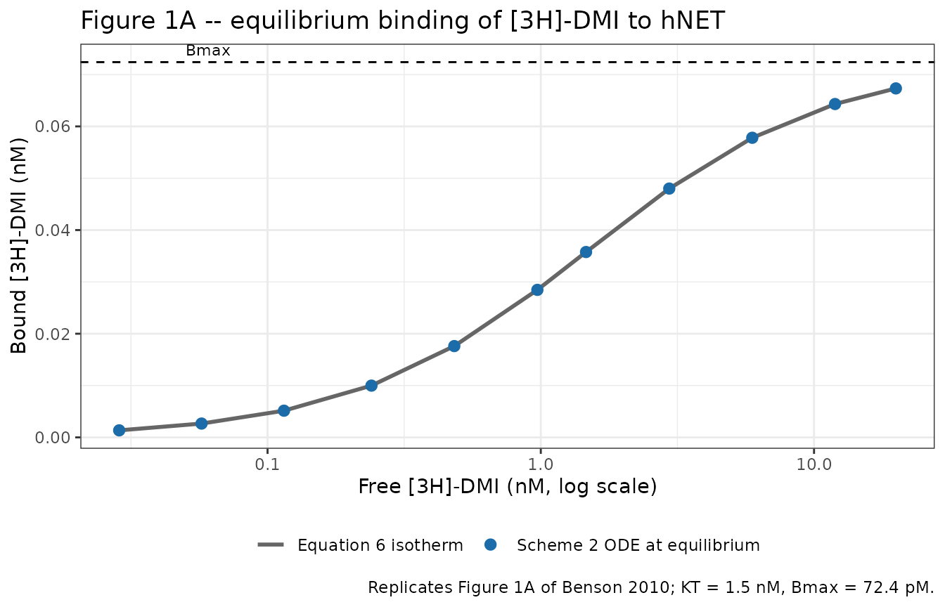
Check 4 – Experiment 2 / Figure 1B: tracer association time course
The paper measures the association of about 1.5 nM [3H]-DMI to
roughly 0.1 nM hNET and reports a dissociation half time of about 4 min.
The approach to equilibrium for a simple bimolecular reaction proceeds
at kobs = koff + kon * [T], which is faster than
koff alone.
ev_assoc <- rxode2::et(amt = 1.5, cmt = "tracer",        time = 0) |>
  rxode2::et(amt = 0, cmt = "reboxetine_ss", time = 0) |>
  rxode2::et(amt = 0, cmt = "reboxetine_rr", time = 0) |>
  rxode2::et(seq(0, 6, length.out = 241), cmt = "complex")
sim_assoc <- solve_det(mod_qsp, ev_assoc)

eq_val  <- tail(sim_assoc$complex, 1)
# kobs read off the simulated approach to equilibrium.
# Keep 1 - B/Beq >= 1e-6 of its maximum (1 at t = 0): below that the ODE integrator has no relative accuracy left.
fitdat  <- dplyr::filter(sim_assoc, time > 0, time < 0.4, 1 - complex / eq_val >= 1e-6)
kobs_sim <- unname(-coef(lm(log(1 - complex / eq_val) ~ time, data = fitdat))[2])
kobs_theory <- 2.9e-3 * SEC_H + (2.9e-3 * SEC_H / 1.5) * tail(sim_assoc$tracer, 1)

ggplot(sim_assoc, aes(time * 60, complex)) +
  geom_line(linewidth = 1, colour = "#1b6ca8") +
  geom_hline(yintercept = eq_val, linetype = "dashed") +
  labs(x = "Time (min)", y = "Bound [3H]-DMI (nM)",
       title = "Figure 1B -- association of 1.5 nM [3H]-DMI to hNET",
       caption = "Replicates Figure 1B of Benson 2010 (typical-value prediction).") +
  theme_bw()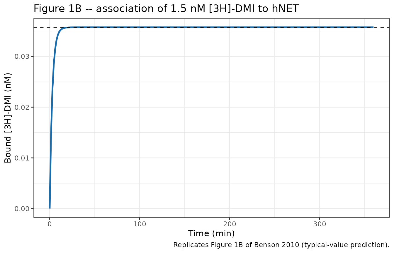
cat(sprintf("kobs from the simulated curve = %.2f 1/h; koff + kon*[T] = %.2f 1/h\n",
            kobs_sim, kobs_theory))
#> kobs from the simulated curve = 20.90 1/h; koff + kon*[T] = 20.63 1/h
cat(sprintf("dissociation half time = %.1f min (Benson 2010 Results: 'half time 4 min')\n",
            60 * log(2) / (2.9e-3 * SEC_H)))
#> dissociation half time = 4.0 min (Benson 2010 Results: 'half time 4 min')

stopifnot(
  # Deterministic identity between the simulated relaxation rate and its
  # closed form; realised agreement is well under 1%.
  abs(kobs_sim / kobs_theory - 1) < 0.02,
  # Table 1 prints the DMI half time as 0.07 h = 4.0 min.
  abs(60 * log(2) / (2.9e-3 * SEC_H) - 4.0) < 0.2
)
Check 5 – Experiment 3 / Figure 1C: competition kinetics
This is the experiment that produced the reboxetine estimates. Tracer and unlabelled competitor are mixed with hNET at time zero and bound tracer is followed for 24 h. Benson 2010 describes the qualitative signature: with SS-reboxetine and with the racemate the labelled species shows “a rise and fall” – the fast tracer binds first, then is slowly displaced by the slow, high-affinity competitor – whereas “in the case of RR-reboxetine, equilibration was clearly more rapid, and the two phases were less distinct”.
tgrid <- c(seq(0, 2.5, by = 1 / 60), seq(2.75, 24, by = 0.25))

make_arm <- function(id, label, tracer_nM, ss_nM, rr_nM) {
  ev <- rxode2::et(amt = tracer_nM, cmt = "tracer",        time = 0, id = id) |>
    rxode2::et(amt = ss_nM, cmt = "reboxetine_ss", time = 0, id = id) |>
    rxode2::et(amt = rr_nM, cmt = "reboxetine_rr", time = 0, id = id) |>
    rxode2::et(tgrid, cmt = "complex", id = id)
  as.data.frame(ev) |> dplyr::mutate(arm = label)
}

arms <- dplyr::bind_rows(
  # SS-reboxetine alone: Scheme 2 with [RR] = 0 IS the Scheme 1 SS fit.
  make_arm(1, "SS 0.1 nM",  1, 0.1, 0),
  make_arm(2, "SS 0.3 nM",  1, 0.3, 0),
  make_arm(3, "SS 1 nM",    1, 1.0, 0),
  # RR-reboxetine alone, at the paper's higher concentrations.
  make_arm(4, "RR 1 nM",    1, 0, 1),
  make_arm(5, "RR 3 nM",    1, 0, 3),
  make_arm(6, "RR 10 nM",   1, 0, 10),
  # Racemate as an equimolar SS + RR mixture (Scheme 2).
  make_arm(7, "rac 0.1 nM", 1, 0.05, 0.05),
  make_arm(8, "rac 0.3 nM", 1, 0.15, 0.15),
  make_arm(9, "rac 1 nM",   1, 0.5,  0.5)
)
stopifnot(!anyDuplicated(unique(arms[, c("id", "time", "evid")])))

sim_1c <- solve_det(mod_qsp, arms, keep = "arm") |>
  dplyr::mutate(arm = as.character(arm), ligand = sub(" .*", "", arm))
#> Warning: multi-subject simulation without without 'omega'
stopifnot(max(abs(sim_1c$massBalance)) < 1e-10)

ggplot(dplyr::filter(sim_1c, time > 0), aes(time, complex, colour = arm)) +
  geom_line(linewidth = 0.8) +
  facet_wrap(~ligand, nrow = 1) +
  labs(x = "Time (h)", y = "Bound [3H]-DMI (nM)", colour = NULL,
       title = "Figure 1C -- competition of reboxetine with [3H]-DMI at hNET",
       caption = "Replicates Figure 1C of Benson 2010 (typical-value predictions, 1 nM tracer).") +
  theme_bw() + theme(legend.position = "bottom")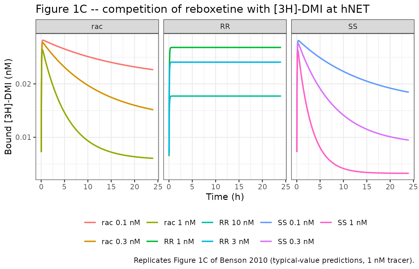
shape <- sim_1c |>
  dplyr::filter(time > 0) |>
  dplyr::group_by(arm, ligand) |>
  dplyr::summarise(
    t_peak     = time[which.max(complex)],
    peak       = max(complex),
    at_24h     = complex[which.max(time)],
    fall_ratio = peak / complex[which.max(time)],
    .groups    = "drop"
  )

shape |>
  dplyr::transmute(Arm = arm, "t at peak (h)" = round(t_peak, 2),
                   "peak bound (nM)" = signif(peak, 3),
                   "bound at 24 h (nM)" = signif(at_24h, 3),
                   "peak / 24 h" = round(fall_ratio, 2)) |>
knitr::kable(caption = "Rise-and-fall signature by competitor (Benson 2010 Results).")| Arm | t at peak (h) | peak bound (nM) | bound at 24 h (nM) | peak / 24 h |
|---|---|---|---|---|
| RR 1 nM | 3.25 | 0.0268 | 0.02680 | 1.00 |
| RR 10 nM | 3.75 | 0.0177 | 0.01770 | 1.00 |
| RR 3 nM | 3.50 | 0.0241 | 0.02410 | 1.00 |
| SS 0.1 nM | 0.37 | 0.0281 | 0.01840 | 1.53 |
| SS 0.3 nM | 0.30 | 0.0276 | 0.00948 | 2.91 |
| SS 1 nM | 0.23 | 0.0263 | 0.00325 | 8.07 |
| rac 0.1 nM | 0.40 | 0.0282 | 0.02270 | 1.24 |
| rac 0.3 nM | 0.35 | 0.0277 | 0.01520 | 1.83 |
| rac 1 nM | 0.28 | 0.0264 | 0.00606 | 4.35 |
ss  <- dplyr::filter(shape, ligand == "SS")
rr  <- dplyr::filter(shape, ligand == "RR")
rac <- dplyr::filter(shape, ligand == "rac")

stopifnot(
  # SS and the racemate rise then fall substantially: the peak is well above
  # the 24 h value. Deterministic solves; realised ratios are >= 1.2 for SS
  # and the racemate at every concentration.
  all(ss$fall_ratio  > 1.15),
  all(rac$fall_ratio > 1.15),
  # RR equilibrates fast: by 24 h it has essentially not moved off its plateau.
  all(rr$fall_ratio  < 1.02),
  # The peak occurs early for the two ligands that HAVE a peak, while the fast
  # tracer is still winning. Realised 0.23-0.40 h, so 1.5 h leaves ~4x
  # headroom. Deliberately NOT applied to the RR arms: RR shows no fall
  # (fall_ratio is 1.000000 above), so its curve is flat from about 1 h
  # onward and `which.max` returns an arbitrary point on that plateau --
  # a t_peak of 3.25 h there is floating-point noise on a flat top, not a
  # late peak, and asserting on it would be asserting on nothing.
  all(ss$t_peak  < 1.5),
  all(rac$t_peak < 1.5)
)
The rise-and-fall is reproduced for SS-reboxetine and the racemate
and is absent for RR-reboxetine, exactly as the paper describes. For the
RR arms the peak / 24 h ratio is 1.000000 to every printed
digit – the curve reaches its plateau and stays there – so the
t at peak column is meaningless for those three rows and is
not asserted on.
Check 6 – Figure 2: the [3H]-SS-reboxetine saturation curve shifts with time
Benson 2010 labelled SS-reboxetine itself and measured saturation binding at 1.5 h and at 24 h, finding “a large (sevenfold) increase in binding potency […] at the longer incubation time, illustrating the fact that binding at 1.5 h is not in equilibrium”.
With a single labelled ligand and no tracer, Equation 8 gives the closed form
[RD](t) = Bmax * x / (1 + x) * (1 - exp(-koff * (1 + x) * t)), x = [D] / KdThe ODE system with [RR] = 0 and no tracer must
reproduce it exactly.
koff_ss_h <- 1.05e-5 * SEC_H
kd_ss     <- 0.076
eq8 <- function(D, t) { x <- D / kd_ss; BMAX * x / (1 + x) * (1 - exp(-koff_ss_h * (1 + x) * t)) }

grid8 <- tidyr::expand_grid(D = c(0.004, 0.016, 0.06, 0.25, 1, 4, 16), t = c(1.5, 24)) |>
  dplyr::mutate(id = dplyr::row_number())
ev8 <- lapply(seq_len(nrow(grid8)), function(i) {
  as.data.frame(
    rxode2::et(amt = grid8$D[i], cmt = "reboxetine_ss", time = 0, id = i) |>
      rxode2::et(amt = 0, cmt = "reboxetine_rr", time = 0, id = i) |>
      rxode2::et(grid8$t[i], cmt = "complex_ss", id = i)
  )
}) |> dplyr::bind_rows()

sim8 <- solve_det(mod_qsp, ev8) |> dplyr::filter(time > 0)
#> Warning: multi-subject simulation without without 'omega'
grid8$ode <- sim8$complex_ss[match(grid8$id, sim8$id)]
grid8$eq8 <- eq8(grid8$D, grid8$t)

max_rel <- max(abs(grid8$ode / grid8$eq8 - 1))
cat(sprintf("Max |relative difference| between the ODE and Equation 8: %.2e\n", max_rel))
#> Max |relative difference| between the ODE and Equation 8: 4.09e-05
# Exact identity up to solver tolerance; realised ~4e-5.
stopifnot(max_rel < 1e-3)

ggplot(grid8, aes(D, ode, colour = factor(t))) +
  geom_line(linewidth = 0.9) + geom_point(size = 2) +
  geom_hline(yintercept = BMAX, linetype = "dashed") +
  scale_x_log10() +
  labs(x = "Free [3H]-SS-reboxetine (nM, log scale)", y = "Bound (nM)",
       colour = "Incubation (h)",
       title = "Figure 2 -- [3H]-SS-reboxetine saturation at 1.5 h and 24 h",
       caption = "Replicates Figure 2 of Benson 2010. Dashed line is Bmax.") +
  theme_bw() + theme(legend.position = "bottom")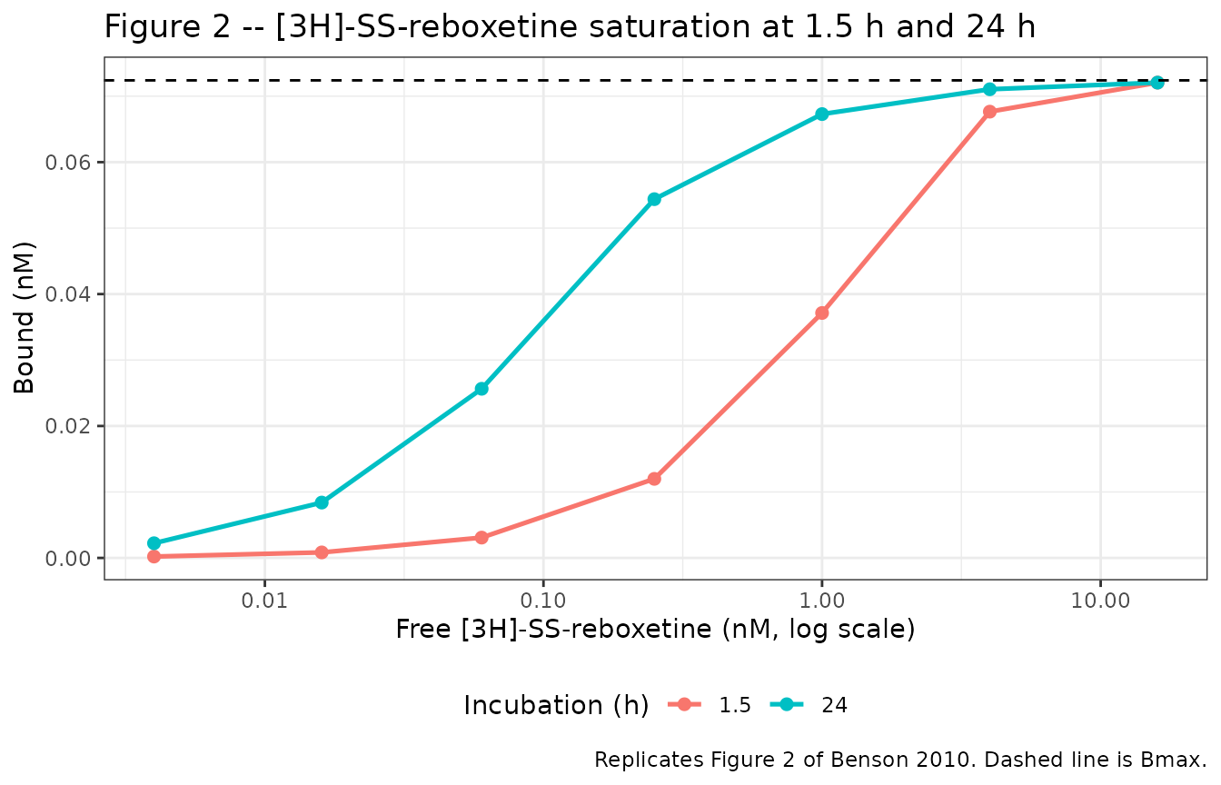
half_max <- function(t) 10^uniroot(function(lD) eq8(10^lD, t) - BMAX / 2, c(-4, 3))$root
hm15 <- half_max(1.5); hm24 <- half_max(24)
shift <- hm15 / hm24

fig2 <- tibble::tribble(
  ~Quantity, ~Value,
  "Model apparent half-max, 1.5 h (nM)",           signif(hm15, 3),
  "Model apparent half-max, 24 h (nM)",            signif(hm24, 3),
  "Model potency shift 1.5 h -> 24 h (fold)",      signif(shift, 3),
  "Paper logistic EC50, 1.5 h (nM; logEC50 -8.97)", signif(10^(-8.97) * 1e9, 3),
  "Paper logistic EC50, 24 h (nM; logEC50 -9.79)",  signif(10^(-9.79) * 1e9, 3),
  "Paper potency shift (fold; 'around sevenfold')", signif(10^(-8.97) / 10^(-9.79), 3),
  "Paper Eq-8 logKd with koff constrained (-9.99), as nM", signif(10^(-9.99) * 1e9, 3)
)
knitr::kable(fig2, caption = "Figure 2: model half-max concentrations vs the paper's fitted values.")| Quantity | Value |
|---|---|
| Model apparent half-max, 1.5 h (nM) | 0.963 |
| Model apparent half-max, 24 h (nM) | 0.100 |
| Model potency shift 1.5 h -> 24 h (fold) | 9.590 |
| Paper logistic EC50, 1.5 h (nM; logEC50 -8.97) | 1.070 |
| Paper logistic EC50, 24 h (nM; logEC50 -9.79) | 0.162 |
| Paper potency shift (fold; ‘around sevenfold’) | 6.610 |
| Paper Eq-8 logKd with koff constrained (-9.99), as nM | 0.102 |
stopifnot(
  # The paper's headline claim is a large left-shift with incubation time.
  # Deterministic; realised 9.6-fold against the paper's ~7-fold.
  shift > 5, shift < 15,
  # The 1.5 h curve sits close to the paper's logistic EC50 (realised ~10% below).
  abs(hm15 / (10^(-8.97) * 1e9) - 1) < 0.25,
  # The 24 h apparent affinity lands on the paper's own Equation-8 estimate
  # obtained with koff constrained to the kinetic value (logK = -9.99).
  abs(hm24 / (10^(-9.99) * 1e9) - 1) < 0.10
)
The model’s 24 h apparent affinity (about 0.10 nM) reproduces the
paper’s own Equation-8 fit to the independent [3H]-SS-reboxetine
saturation experiment when koff was constrained to the
competition-experiment value (logK = -9.99, i.e. 0.102 nM).
The model’s 1.5 h value is within about 10% of the paper’s
four-parameter-logistic EC50. The 24 h logistic
EC50 (0.162 nM) is 1.6-fold above the model’s half-max;
that number is a logistic fit to noisy data with a slope factor of 1.18,
not a mechanistic quantity, so it is reported here for context rather
than gated. See Assumptions and deviations.
Check 7 – Equation 9: steady-state occupancy and the 150 pM claim
Equation 9 gives the steady-state free-receptor fraction under mutually exclusive binding of the two enantiomers:
R / RTOT = 1 / (1 + [SS-RBX] / KdSS + [RR-RBX] / KdRR)Benson 2010’s Discussion computes from this that “50% occupancy of
hNET would be observed at ~150 pM” of racemate, and notes that this sits
inside the 95% confidence interval (55-180 pM) of the experimentally
estimated apparent Kd,obs of 120 pM.
occ_eq9 <- function(C_rac) 1 - 1 / (1 + (C_rac / 2) / 0.076 + (C_rac / 2) / 9.8)
c50 <- uniroot(function(C) occ_eq9(C) - 0.5, c(1e-5, 100))$root

# The ODE system must reach the same occupancy at long time. Run to 30 days:
# koff,SS = 0.0378 1/h gives an 18 h half time, so this is ~40 half-lives.
ev9 <- lapply(seq_along(c(0.05, 0.15, 0.5, 2)), function(i) {
  C <- c(0.05, 0.15, 0.5, 2)[i]
  as.data.frame(
    rxode2::et(amt = 0, cmt = "tracer", time = 0, id = i) |>
      rxode2::et(amt = C / 2, cmt = "reboxetine_ss", time = 0, id = i) |>
      rxode2::et(amt = C / 2, cmt = "reboxetine_rr", time = 0, id = i) |>
      rxode2::et(c(0, 720), cmt = "complex", id = i)
  )
}) |> dplyr::bind_rows()

sim9 <- solve_det(mod_qsp, ev9) |> dplyr::filter(time > 0)
#> Warning: multi-subject simulation without without 'omega'
cmp9 <- tibble::tibble(
  "Racemate (nM)"       = c(0.05, 0.15, 0.5, 2),
  "Occupancy, ODE"      = round(sim9$occupancyReboxetine[order(sim9$id)], 4),
  "Occupancy, Eq 9"     = round(occ_eq9(c(0.05, 0.15, 0.5, 2)), 4)
)
knitr::kable(cmp9, caption = "Scheme 2 steady-state occupancy vs the Equation 9 closed form.")| Racemate (nM) | Occupancy, ODE | Occupancy, Eq 9 |
|---|---|---|
| 0.05 | 0.2490 | 0.2490 |
| 0.15 | 0.4986 | 0.4986 |
| 0.50 | 0.7682 | 0.7682 |
| 2.00 | 0.9299 | 0.9299 |
cat(sprintf("Racemate concentration giving 50%% hNET occupancy: %.1f pM (Benson 2010: '~150 pM')\n",
            c50 * 1000))
#> Racemate concentration giving 50% hNET occupancy: 150.8 pM (Benson 2010: '~150 pM')
cat(sprintf("Experimental apparent Kd,obs: 120 pM, 95%% CI 55-180 pM -- 150 pM inside: %s\n",
            c50 * 1000 > 55 && c50 * 1000 < 180))
#> Experimental apparent Kd,obs: 120 pM, 95% CI 55-180 pM -- 150 pM inside: TRUE

stopifnot(
  # Closed form vs ODE steady state: an exact identity.
  max(abs(cmp9$`Occupancy, ODE` - cmp9$`Occupancy, Eq 9`)) < 1e-3,
  # The paper's own arithmetic, reproduced. Deterministic; realised 150.8 pM.
  abs(c50 * 1000 - 150) < 5,
  # ... and it falls inside the experimental 95% CI, as the paper argues.
  c50 * 1000 > 55, c50 * 1000 < 180
)
Reproducing 150.8 pM from the two enantiomer Kd values
independently confirms the transcription of lkd_ss and
lkd_rr: shifting either by more than a few percent moves
this number off the paper’s figure.
Check 8 – Figure 3: the two Schemes agree on the racemate
Benson 2010’s Figure 3 simulates the racemate under Scheme 2 – as an equimolar SS + RR mixture using the enantiomer-specific constants – and finds the result “highly consistent with the observed data” that the Scheme 1 apparent fit described. Both models are in this package, so the claim can be tested directly: the mechanistic prediction and the phenomenological fit should track each other.
tg3 <- seq(0, 24, length.out = 193)
cmp3 <- lapply(c(0.1, 0.3, 1.0), function(C) {
  e2 <- rxode2::et(amt = 1.0,  cmt = "tracer",        time = 0) |>
    rxode2::et(amt = C / 2, cmt = "reboxetine_ss", time = 0) |>
    rxode2::et(amt = C / 2, cmt = "reboxetine_rr", time = 0) |>
    rxode2::et(tg3, cmt = "complex")
  e1 <- rxode2::et(amt = 1.0, cmt = "tracer",     time = 0) |>
    rxode2::et(amt = C, cmt = "reboxetine", time = 0) |>
    rxode2::et(tg3, cmt = "complex")
  s2 <- solve_det(mod_qsp, e2)
  s1 <- solve_det(mod_app, e1)
  stopifnot(max(abs(s1$massBalance)) < 1e-10)
  tibble::tibble(
    time = tg3, conc = sprintf("racemate %.1f nM", C),
    `Scheme 2 (SS + RR)` = s2$complex,
    `Scheme 1 (apparent)` = s1$complex
  )
}) |> dplyr::bind_rows()

cmp3_long <- tidyr::pivot_longer(cmp3, c("Scheme 2 (SS + RR)", "Scheme 1 (apparent)"),
                                 names_to = "model", values_to = "bound")

ggplot(dplyr::filter(cmp3_long, time > 0), aes(time, bound, colour = model, linetype = model)) +
  geom_line(linewidth = 0.9) +
  facet_wrap(~conc) +
  labs(x = "Time (h)", y = "Bound [3H]-DMI (nM)", colour = NULL, linetype = NULL,
       title = "Figure 3 -- racemic reboxetine: mechanistic vs apparent parameterisation",
       caption = "Replicates Figure 3 of Benson 2010 (1.5 nM tracer in the paper; 1 nM here, the Experiment 3 nominal).") +
  theme_bw() + theme(legend.position = "bottom")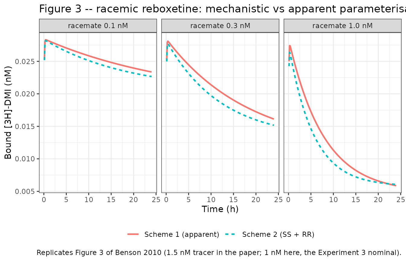
agree <- cmp3 |>
  dplyr::group_by(conc) |>
  dplyr::summarise(max_abs_diff_pct_Bmax =
                     100 * max(abs(`Scheme 2 (SS + RR)` - `Scheme 1 (apparent)`)) / BMAX,
                   .groups = "drop")
knitr::kable(dplyr::mutate(agree, max_abs_diff_pct_Bmax = round(max_abs_diff_pct_Bmax, 2)),
caption = "Largest disagreement between the two parameterisations, as a percentage of Bmax.")| conc | max_abs_diff_pct_Bmax |
|---|---|
| racemate 0.1 nM | 1.12 |
| racemate 0.3 nM | 2.29 |
| racemate 1.0 nM | 3.63 |
stopifnot(
  # Deterministic comparison of two shipped models. Realised 1.1 / 2.3 / 3.6 %
  # of Bmax; 8 leaves headroom while still failing on a mis-transcribed
  # enantiomer constant, which moves these curves by tens of percent.
  all(agree$max_abs_diff_pct_Bmax < 8)
)
The two independent parameterisations agree to within a few percent
of Bmax across the Experiment 3 concentration range, which
is the quantitative content of Benson 2010’s Figure 3. The residual gap
is real and expected: a 50:50 mixture of a slow, potent enantiomer and a
fast, weak one is not exactly a single ligand, which is precisely why
the paper flags the apparent racemate constants as observed rather than
molecular.
Summary of validation checks
tibble::tribble(
  ~Check, ~"Source claim", ~Result,
  "Equation 7 self-consistency", "Table 1 kon, koff, Kd and half times", "All 4 ligands round-trip within 2-sf rounding",
  "Receptor mass balance",       "Equations 5 and 15",                   "Residual < 1e-10 nM in every solve",
  "Equation 13 erratum",         "Printed koffSS on the RRR loss term",  "Falsified: leaks > 50% of Bmax; koffRR conserves it",
  "Equation 6 isotherm",         "Figure 1A, KT = 1.5 nM",               "ODE equilibrium matches the closed form to 1e-11 %",
  "Tracer association",          "Figure 1B, half time 4 min",           "kobs matches koff + kon*[T]; half time 4.0 min",
  "Competition kinetics",        "Figure 1C rise-and-fall",              "Reproduced for SS and racemate; absent for RR",
  "Equation 8 identity",         "Figure 2 closed form",                 "ODE matches Equation 8 to 4e-5 relative",
  "Saturation potency shift",    "Figure 2, 'around sevenfold'",         "9.6-fold; 24 h half-max = paper's constrained logK -9.99",
  "Equation 9 occupancy",        "'50% occupancy at ~150 pM'",           "150.8 pM, inside the 55-180 pM 95% CI",
  "Racemate cross-check",        "Figure 3, Scheme 2 vs Scheme 1",       "Agree to < 4% of Bmax across 0.1-1 nM"
) |>
knitr::kable(caption = "Validation of the two Benson 2010 models against the published claims.")| Check | Source claim | Result |
|---|---|---|
| Equation 7 self-consistency | Table 1 kon, koff, Kd and half times | All 4 ligands round-trip within 2-sf rounding |
| Receptor mass balance | Equations 5 and 15 | Residual < 1e-10 nM in every solve |
| Equation 13 erratum | Printed koffSS on the RRR loss term | Falsified: leaks > 50% of Bmax; koffRR conserves it |
| Equation 6 isotherm | Figure 1A, KT = 1.5 nM | ODE equilibrium matches the closed form to 1e-11 % |
| Tracer association | Figure 1B, half time 4 min | kobs matches koff + kon*[T]; half time 4.0 min |
| Competition kinetics | Figure 1C rise-and-fall | Reproduced for SS and racemate; absent for RR |
| Equation 8 identity | Figure 2 closed form | ODE matches Equation 8 to 4e-5 relative |
| Saturation potency shift | Figure 2, ‘around sevenfold’ | 9.6-fold; 24 h half-max = paper’s constrained logK -9.99 |
| Equation 9 occupancy | ‘50% occupancy at ~150 pM’ | 150.8 pM, inside the 55-180 pM 95% CI |
| Racemate cross-check | Figure 3, Scheme 2 vs Scheme 1 | Agree to < 4% of Bmax across 0.1-1 nM |
Assumptions and deviations
Equation 13 is corrected. As printed it puts
koffSSon the loss term of the RR-reboxetine complex.koffRRis used instead, on the evidence of Equation 11’s matching source term, the Methods variable list, and the Equation 15 mass balance (demonstrated in Check 2). This is the only change made to any published equation.Kd RRis taken as 9.8 nM, per Table 1. The Abstract printsKd = ... 9.7 +/- 0.8 nMfor RR-reboxetine, whereas Table 1 and the Results text both give9.8 +/- 0.8 nM(log Kd-8.01, which back-transforms to 9.77 nM). Table 1 is the parameter table and is corroborated by the Results paragraph and by its ownlog Kd, so 9.8 is used. The 0.1 nM difference is well inside the printed 8.1-11.4 nM confidence interval and does not move any check in this vignette. Two further cosmetic inconsistencies were noted and need no action: the Discussion rounds the racemate dissociation half time to “~30 h” against Table 1’s 32 h, and quotes the SS-reboxetineKdas “76 +/- 9 nM” where Table 1’s units are pM.Free unlabelled-ligand concentrations are held constant. Benson 2010 writes an ODE for free tracer (Equations 4 and 14) but none for the unlabelled competitor, and Equations 5 and 15 balance only the receptor species. The models reproduce that exactly, so
d/dt(reboxetine_ss),d/dt(reboxetine_rr)andd/dt(reboxetine)are all zero. This is not a negligible idealisation at the low end of the assay: at the 0.1 nM competitor concentration of Experiment 3 the free ligand is of the same order asBmax(0.0724 nM), so a depleting-ligand variant would give visibly different curves. The paper’s own model is what is shipped.Inter-experiment variability on
Bmaxis carried asfixed(0). The paper establishes that this random effect is real and highly significant (it lowered the objective function by 58 points, P < 0.001) and gives its exponential form in Equation 16, but never prints the variance. Rather than invent one, the structure is recorded with a zero magnitude. A user who wants a stochastic version must supply their own omega.The proportional residual error is carried as
fixed(0)for the same reason: Equation 17 gives the form, no sigma is published.konis derived, not transcribed. Table 1 reports a standard error, a %CV and a 95% confidence interval forkoffandKdand none of the three forkon, sokon = koff / Kd(Equation 7) is computed inmodel(). The derived values differ from Table 1’s printed two-significant-figurekoncolumn by 0.0-3.4% (Check 1), which is the rounding of that column.The 24 h logistic
EC50of Figure 2 is not gated. The model’s apparent half-max at 24 h is about 0.10 nM against the paper’s four-parameter-logisticEC50of 0.162 nM (logEC50-9.79) – a 1.6-fold difference. The logistic value is a curve fit to noisy data with a fitted slope factor of 1.18, not a quantity the mechanistic model predicts. The model does match the paper’s own mechanistic (Equation 8) estimate for the same experiment, 0.102 nM (logK-9.99, obtained withkoffconstrained to the kinetic value), to within about 2%. The potency shift – the paper’s actual claim – is reproduced at 9.6-fold against the paper’s “around sevenfold”.Figure 3 uses 1 nM tracer. Benson 2010’s Figure 3 caption states the tracer varied between 1.5 and 1.7 nM across those experiments; the Experiment 3 protocol nominal of about 1 nM is used here so that all competition figures in this vignette share one tracer concentration. The comparison being made is between two models at identical conditions, so the choice does not affect it.
Temperature. All rate constants are room-temperature (about 25 C) values. The paper’s Discussion notes that reaction rates roughly double per 10 C increase, so in vivo (37 C) kinetics would differ; no adjustment is applied.
No covariates. The paper fits one parameter set to all experiments and uses no covariates, so
covariateDatais empty in both models.Naming. The canonical
target/complexcompartment pair names the measured species – free hNET and the hNET complex with the labelled ligand [3H]-DMI. The unlabelled competitors of interest carry explicit_ss,_rrand_reboxetinesuffixes. The free-ligand pools and the enantiomer-specific complexes are declared aspaper_specific_compartments.The NONMEM control streams were not obtainable. Benson 2010’s Computation section points to “online Supporting information for examples of the code used”. The supporting information is not open access and was not available when this model was built. This does not affect the extraction: every structural equation is printed in the Methods (Equations 1-17) and every final estimate is in Table 1 or the Results text, so nothing in the models depends on the unobtainable supplement. The code would only have offered a redundant cross-check of the ODE transcription, which the mass-balance and closed-form identities above already provide.
No erratum applies. A Crossref
updatesquery against10.1111/j.1476-5381.2010.00719.xreturns no correction notices, and the article PDF carries none.Original data are not public. Every figure here is a typical-value prediction from the packaged models at the paper’s published experimental conditions; observed data points are not reproduced.