Tepotinib (Hu 2025) • nlmixr2lib

Model and source

Citation: Hu J, Zhao Y, Rao Q, Li G, Jiao Z, Wang H, Qu Y, Xu S, Gu Z, Wang T, Chen Z, Zhao C, Zhou G. Combining mechanistic quantitative systems pharmacology modeling and patient-derived organoid testing in MET-aberrant non-small cell lung cancer for high-throughput combination efficacy analysis and personalized treatment design. Front Pharmacol. 2025;16:1685468. doi:10.3389/fphar.2025.1685468. PMCID PMC12682884. The model definition is in Supplementary Table S1 (Table1.xlsx; Species, Reactions and Parameters sheets) and Supplementary Figures S4/S9 (DataSheet1.pdf). The tepotinib PK parameters of Supplementary Table S1 are themselves cited to Johne A, Scheible H, Becker A, van Lier JJ, Wolna P, Meyring M. Invest New Drugs. 2020;38(5):1507-1519. doi:10.1007/s10637-020-00926-1 (PMID 32221754), which is not on disk for this extraction.
Article: https://doi.org/10.3389/fphar.2025.1685468
Supplement: https://www.frontiersin.org/articles/10.3389/fphar.2025.1685468/full#supplementary-material (Table1.xlsx = Supplementary Table S1, with Species, Reactions and Parameters sheets; DataSheet1.pdf = Supplementary Figures S1-S9)

Hu 2025 is a quantitative systems pharmacology (QSP) model of MET-aberrant non-small cell lung cancer: roughly 130 species and 69 reactions covering the MET, EGFR, ALK and ROS1 signalling network, three tumour-cell clones, and pharmacokinetic submodules for 16 drugs. Only the human tepotinib PK submodule is packaged here. The signalling and tumour-growth network is not integrable from the published supplement – seven quantities that the printed rate laws consume are reported nowhere (listed under Assumptions and deviations) – and is deferred pending author correspondence.

This vignette has two jobs, and it is important not to confuse them.

It verifies that the packaged model is a faithful, self-consistent transcription of the tepotinib PK module printed in Supplementary Table S1. Those checks pass.
It documents a contradiction inside the publication itself: the printed parameter set does not reproduce the paper’s own human tepotinib simulation in Supplementary Figure S4F. That check fails, by design, and the failure is reported rather than repaired.

No parameter in the packaged model was fitted, tuned, or inferred. Every value is transcribed from Supplementary Table S1. Read the Assumptions and deviations section before using this model to predict tepotinib exposure.

Population

The QSP framework was calibrated across cell lines, mouse xenografts and human trial data, and applied at the clinical level to two virtual-patient cohorts of 5000 subjects each – one representing NSCLC with MET exon 14 skipping mutations, one representing MET amplification (Results, QSP model-based virtual clinical trials). Virtual clinical trials were run against the reported regimens of NCT02414139 (capmatinib), NCT02864992 (tepotinib) and NCT00585195 (crizotinib).

The tepotinib PK submodule itself is a typical-value, deterministic model: the paper reports no between-subject variance and no residual-error model for any of its PK modules. All five printed tepotinib PK parameters are attributed in Supplementary Table S1 to Johne 2020 (PMID 32221754), a phase I mass-balance and absolute-bioavailability study in healthy volunteers. That paper is not on disk for this extraction, so the values were taken as printed and could not be checked against their own cited source.

The clinically approved regimen simulated in Figure 7B is 500 mg once daily (containing 450 mg active moiety); 600 mg QD was also simulated and gave no further gain in objective response rate.

The same information is available programmatically via readModelDb("Hu_2025_tepotinib")()$population.

Source trace

Every entry below is transcribed from Supplementary Table S1. The Parameters sheet gives values and provenance; the Reactions sheet gives the rate laws; the Species sheet gives the compartment assignment.

Model term	Value	Source location
`lka` (ka)	0.2 1/h	`Parameters` sheet, `ka_tepo = 0.2 (hour^-1)`, ref PMID 32221754
`lcl` (CL/F)	44.88 L/h	`Parameters` sheet, `kcl_tepo = 1.32 (hour^-1)` times `Vc = 34 (L)`; v68 applies `kcl_tepo` to the central amount, so CL = `kcl_tepo` x `Vc`
`lvc` (Vc/F)	34 L	`Parameters` sheet, `Vc = 34 (L)`, ref PMID 32221754
`lq` (Q/F)	1.32 L/h	`Parameters` sheet, `Q = 1.32 (L*hour^-1)`, ref PMID 32221754
`lvp` (Vp/F)	726.8 L	`Parameters` sheet, `vp_tepo = 726.8 (L)`, ref PMID 32221754
`lfdepot` (F)	1	`Reactions` sheet, v67 carries no bioavailability term
`propSd`	0	No residual-error model reported anywhere in the paper or supplement
`d/dt(depot)`	n/a	v67, `ka_tepo*tepo_dose`
elimination term of `d/dt(central)`	n/a	v68, `kcl_tepo*tepo_c`
distribution terms of `d/dt(central)`, `d/dt(peripheral1)`	n/a	v69 (see Assumptions and deviations: the printed divisors are transposed and the mass-conserving form is encoded)
two-compartment structure	n/a	`Reactions` sheet footnote, “two-compartment (for tepotinib) clinical pharmacokinetic (PK) module”; `Species` sheet assigns `tepo_c` to central and `tepo_p` to peripheral
`Cc <- central / vc`	n/a	`Species` sheet, `tepo_c` in the central compartment

The packaged model

mod <- readModelDb("Hu_2025_tepotinib")
#> ℹ Parameters are transcribed verbatim from Supplementary Table S1, but that printed set does NOT reproduce the paper's own human tepotinib simulation in Supplementary Figure S4F: terminal half-life 393 h vs about 29 h in the figure, and roughly 60-fold low over 13-199 h. The contradiction is internal to the publication and is documented, not repaired. See the validation vignette before using this model to predict tepotinib exposure.

DOSE_MG      <- 500      # Supplementary Figure S4F legend; approved dose, Figure 7B
MW_TEPOTINIB <- 492.58   # g/mol, tepotinib free base (C29H28N6O2)

# ug/mL (= mg/L) -> mol/L, to plot on the axis Supplementary Figure S4F uses.
as_molar <- function(conc_ug_per_mL) conc_ug_per_mL / 1000 / MW_TEPOTINIB

# A fine early grid resolves the sharp absorption peak (tmax is under 2 h);
# the coarse tail runs to about 7.6 terminal half-lives so that AUC(0-Inf)
# needs almost no extrapolation.
obs_grid <- c(seq(0, 24, by = 0.05), seq(24.5, 3000, by = 0.5))

ev_single <- rxode2::et(amt = DOSE_MG, cmt = "depot") |>
  rxode2::et(obs_grid)

sim_single <- rxode2::rxSolve(mod, ev_single) |>
  as.data.frame() |>
  dplyr::mutate(conc_M = as_molar(Cc))

sim_200 <- dplyr::filter(sim_single, time <= 200)

ggplot(sim_200, aes(time, conc_M)) +
  geom_line(linewidth = 0.8, colour = "firebrick") +
  scale_y_log10() +
  labs(x = "Time (h)", y = "Plasma tepotinib (mol/L)",
       title = "Packaged model, tepotinib 500 mg single oral dose",
       subtitle = "Parameters exactly as printed in Supplementary Table S1")
#> Warning in scale_y_log10(): log-10 transformation introduced infinite values.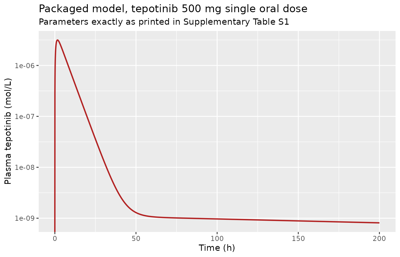

Packaged model: tepotinib 500 mg single oral dose, plotted over the 0-200 h window of Supplementary Figure S4F.

Structural identity checks

These compare the solved model against its own closed form. Both sides use the same parameters, so the discrepancy is pure numerical error and a tight bound is the correct assertion.

# Printed parameters, restated here so the identities are checked against the
# source numbers rather than against whatever the model file happens to hold.
KA  <- 0.2         # ka_tepo, 1/h
KCL <- 1.32        # kcl_tepo, 1/h
VC  <- 34          # Vc, L
Q   <- 1.32        # Q, L/h
VP  <- 726.8       # vp_tepo, L
CL  <- KCL * VC    # 44.88 L/h

# (a) Model file agrees with the printed values.
prm <- rxode2::rxode(mod)$theta
stopifnot(
  abs(exp(prm[["lka"]]) - KA)  < 1e-10,
  abs(exp(prm[["lcl"]]) - CL)  < 1e-10,
  abs(exp(prm[["lvc"]]) - VC)  < 1e-10,
  abs(exp(prm[["lq"]])  - Q)   < 1e-10,
  abs(exp(prm[["lvp"]]) - VP)  < 1e-10
)

# (b) The peripheral compartment is really there. rxSolve() defaults to
# useLinCmt = TRUE, which can silently collapse a two-compartment system
# written with micro-constants down to one compartment; the give-away is a
# terminal half-life equal to log(2)/kel. Assert the analytic beta root of
# x^2 - (kel + k12 + k21)x + kel*k21 = 0 instead.
kel <- CL / VC; k12 <- Q / VC; k21 <- Q / VP
sroot   <- kel + k12 + k21
beta    <- (sroot - sqrt(sroot^2 - 4 * kel * k21)) / 2
thalf_z <- log(2) / beta

tail_dat  <- dplyr::filter(sim_single, time >= 1500)
slope_fit <- lm(log(Cc) ~ time, data = tail_dat)
thalf_sim <- log(2) / -unname(coef(slope_fit)[2])

stopifnot(
  abs(thalf_sim / thalf_z - 1) < 1e-3,
  # ... and it is emphatically NOT the one-compartment answer.
  thalf_sim / (log(2) / kel) > 100
)

# (c) With F = 1, AUC(0-Inf) must equal Dose / CL exactly.
nca_single <- PKNCA::pk.nca(PKNCA::PKNCAdata(
  PKNCA::PKNCAconc(
    sim_single |>
      dplyr::filter(!is.na(Cc)) |>
      dplyr::transmute(id = 1L, treatment = "500 mg single oral dose", time, Cc),
    Cc ~ time | treatment + id
  ),
  PKNCA::PKNCAdose(
    tibble::tibble(id = 1L, treatment = "500 mg single oral dose",
                   time = 0, amt = DOSE_MG),
    amt ~ time | treatment + id
  ),
  intervals = data.frame(start = 0, end = Inf,
                         cmax = TRUE, tmax = TRUE,
                         aucinf.obs = TRUE, half.life = TRUE)
))

nca_val <- function(res, code) {
  as.data.frame(res) |>
    dplyr::filter(PPTESTCD == code) |>
    dplyr::pull(PPORRES)
}

auc_inf <- nca_val(nca_single, "aucinf.obs")
stopifnot(abs(auc_inf / (DOSE_MG / CL) - 1) < 1e-3)

# (d) Mass balance. The distribution flux v69 is encoded in its mass-conserving
# form, so at any time the dose must equal drug still in the body plus drug
# eliminated, and eliminated drug is exactly CL times AUC(0-t).
t_chk    <- 500
state    <- dplyr::filter(sim_single, time == t_chk)
in_body  <- state$depot + state$central + state$peripheral1
auc_0_t  <- PKNCA::pk.calc.auc(
  dplyr::filter(sim_single, time <= t_chk)$Cc,
  dplyr::filter(sim_single, time <= t_chk)$time,
  interval = c(0, t_chk)
)
stopifnot(abs((in_body + CL * auc_0_t) / DOSE_MG - 1) < 1e-3)

c(terminal_half_life_h  = signif(thalf_sim, 4),
  analytic_beta_root_h  = signif(thalf_z, 4),
  one_cmt_half_life_h   = signif(log(2) / kel, 4),
  auc_inf_mg_h_per_L    = signif(auc_inf, 5),
  dose_over_cl          = signif(DOSE_MG / CL, 5),
  mass_balance_fraction = signif((in_body + CL * auc_0_t) / DOSE_MG, 6))
#>  terminal_half_life_h  analytic_beta_root_h   one_cmt_half_life_h 
#>             392.90000             392.90000               0.52510 
#>    auc_inf_mg_h_per_L          dose_over_cl mass_balance_fraction 
#>              11.14000              11.14100               0.99994

The terminal half-life implied by the printed parameters is 393 h – more than 100-fold longer than the 0.53 h half-life of the central compartment alone, because Q = 1.32 L/h returns drug from a 726.8 L peripheral volume with a rate constant of only 0.00182 1/h. Hold on to that number; the next section shows the paper’s own figure is inconsistent with it.

PKNCA validation

as.data.frame(nca_single) |>
  dplyr::mutate(PPORRES = signif(PPORRES, 4)) |>
  dplyr::select(treatment, PPTESTCD, PPORRES) |>
  dplyr::rename("Regimen" = treatment, "Parameter" = PPTESTCD, "Value" = PPORRES) |>
  knitr::kable(caption = paste(
    "PKNCA on the packaged model, 500 mg single oral dose.",
    "Concentrations in ug/mL, time in h."
  ))

PKNCA on the packaged model, 500 mg single oral dose. Concentrations in ug/mL, time in h.
Regimen	Parameter	Value
500 mg single oral dose	cmax	1.555e+00
500 mg single oral dose	tmax	1.650e+00
500 mg single oral dose	tlast	3.000e+03
500 mg single oral dose	clast.obs	2.900e-06
500 mg single oral dose	lambda.z	1.766e-03
500 mg single oral dose	r.squared	9.999e-01
500 mg single oral dose	adj.r.squared	9.999e-01
500 mg single oral dose	lambda.z.time.first	4.550e+01
500 mg single oral dose	lambda.z.time.last	3.000e+03
500 mg single oral dose	lambda.z.n.points	5.910e+03
500 mg single oral dose	clast.pred	2.900e-06
500 mg single oral dose	half.life	3.925e+02
500 mg single oral dose	span.ratio	7.527e+00
500 mg single oral dose	aucinf.obs	1.114e+01

Steady state on the approved 500 mg QD regimen

Figure 7B of the paper simulates tepotinib 500 mg once daily. A 393 h terminal half-life against a 24 h dosing interval would normally imply heavy accumulation – but it does not here, and the reason is worth spelling out.

# 125 doses = 2976 h of dosing, about 7.6 terminal half-lives.
ev_qd <- rxode2::et(amt = DOSE_MG, cmt = "depot", ii = 24, addl = 124) |>
  rxode2::et(obs_grid)

sim_qd   <- rxode2::rxSolve(mod, ev_qd) |> as.data.frame()
last_tau <- dplyr::filter(sim_qd, time >= 2976, time <= 3000)
first_24 <- dplyr::filter(sim_single, time <= 24)

auc_tau  <- PKNCA::pk.calc.auc(last_tau$Cc, last_tau$time,
                               interval = c(2976, 3000))
auc_sd24 <- PKNCA::pk.calc.auc(first_24$Cc, first_24$time,
                               interval = c(0, 24))

# At steady state, AUC over one dosing interval must equal Dose / CL.
stopifnot(abs(auc_tau / (DOSE_MG / CL) - 1) < 0.02)

# The 393 h terminal phase carries almost no exposure: a single dose has
# already delivered the great majority of AUC(0-Inf) within the first 24 h,
# so accumulation on a daily regimen is negligible despite that half-life.
stopifnot(
  auc_sd24 / auc_inf > 0.9,
  abs(auc_tau / auc_sd24 - 1) < 0.1
)

c(auc_tau_mg_h_per_L   = signif(auc_tau, 5),
  dose_over_cl         = signif(DOSE_MG / CL, 5),
  auc_accumulation     = signif(auc_tau / auc_sd24, 3),
  cmax_accumulation    = signif(max(last_tau$Cc) / max(sim_single$Cc), 3),
  ctrough_accumulation = signif(min(last_tau$Cc) /
                                 sim_single$Cc[sim_single$time == 24], 3),
  frac_auc_in_first_24h = signif(auc_sd24 / auc_inf, 3))
#>    auc_tau_mg_h_per_L          dose_over_cl      auc_accumulation 
#>                11.073                11.141                 1.030 
#>     cmax_accumulation  ctrough_accumulation frac_auc_in_first_24h 
#>                 1.010                 1.590                 0.963

Accumulation is 1.03-fold on AUC and 1.01-fold on Cmax; only the trough moves appreciably, by 1.59-fold. The 393 h terminal phase is real but carries almost no drug: 96% of AUC(0-Inf) is delivered in the first 24 h, because Q = 1.32 L/h moves only a small fraction of the dose into the peripheral compartment before kcl_tepo has cleared the rest. So the printed parameter set produces a tall, narrow spike with a long low-amplitude tail – which is exactly the shape Supplementary Figure S4F does not show.

ggplot(sim_qd, aes(time / 24, Cc)) +
  geom_line(linewidth = 0.6) +
  labs(x = "Time (days)", y = "Plasma tepotinib (ug/mL)",
       title = "Tepotinib 500 mg QD to steady state",
       subtitle = "Printed Supplementary Table S1 parameters")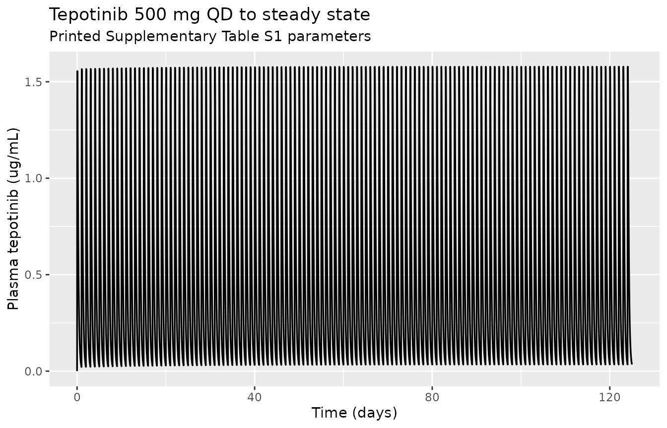

Tepotinib 500 mg QD, the approved regimen simulated in Figure 7B of Hu 2025, as the packaged model predicts it.

The printed parameters do not reproduce Supplementary Figure S4F

This is the finding this vignette exists to record.

Supplementary Figure S4 panel F is the paper’s own human tepotinib simulation: “tepotinib (500 mg, single oral dose)”, a red simulation trace with published human PK data overlaid, plotted as molar plasma concentration on a log axis over 0-200 h. The trace below was read off a render of that panel at extraction time; the axis calibration comes from the printed decade labels and the 0 / 100 / 200 hour ticks. The 86-110 h region is omitted because the legend box overlaps the trace there. Read-off uncertainty is roughly 10%, dominated by log-axis gridline resolution – immaterial at the scale of the discrepancy below.

figS4F <- tibble::tibble(
  time = c(13, 15, 18, 20, 25, 30, 35, 40, 50, 60,
           70, 80, 113, 120, 130, 140, 150, 165, 180, 199),
  conc_M = c(1.216e-06, 1.216e-06, 1.070e-06, 1.070e-06, 1.070e-06,
             8.504e-07, 8.447e-07, 8.166e-07, 5.986e-07, 4.477e-07,
             3.238e-07, 2.574e-07, 1.225e-07, 1.152e-07, 8.222e-08,
             6.535e-08, 5.710e-08, 3.583e-08, 2.522e-08, 1.705e-08)
)

# Terminal slope read straight off the figure trace (t >= 113 h).
fig_tail  <- lm(log(conc_M) ~ time, data = dplyr::filter(figS4F, time >= 113))
thalf_fig <- log(2) / -unname(coef(fig_tail)[2])
c(figure_terminal_half_life_h = signif(thalf_fig, 3),
  printed_terminal_half_life_h = signif(thalf_z, 4))
#>  figure_terminal_half_life_h printed_terminal_half_life_h 
#>                         29.3                        392.9

The figure declines log-linearly with a terminal half-life of about 29.3 h. The printed parameters imply 393 h. That alone settles the matter: no choice of ka can reconcile a 393 h terminal slope with a 29.3 h one, because the terminal slope is a property of the disposition parameters only.

cmp_pts <- tibble::tibble(
  time      = figS4F$time,
  predicted = approx(sim_single$time, sim_single$conc_M, xout = figS4F$time)$y,
  figure    = figS4F$conc_M
) |>
  dplyr::mutate(ratio = predicted / figure)

stopifnot(
  # The packaged model sits below the paper's own figure at every read-off
  # point, by between roughly 3-fold and several hundred-fold. Asserting the
  # finding keeps it from silently drifting if rxode2 changes.
  all(cmp_pts$ratio < 1),
  exp(mean(log(cmp_pts$ratio))) < 0.05,
  max(1 / cmp_pts$ratio) > 100
)

c(geometric_mean_ratio = signif(exp(mean(log(cmp_pts$ratio))), 3),
  worst_fold_low       = signif(max(1 / cmp_pts$ratio), 4),
  best_fold_low        = signif(min(1 / cmp_pts$ratio), 3))
#> geometric_mean_ratio       worst_fold_low        best_fold_low 
#>               0.0169             464.1000               3.1700

ggplot(sim_200, aes(time, conc_M)) +
  geom_line(linewidth = 0.8, colour = "firebrick") +
  geom_point(data = figS4F, aes(time, conc_M), inherit.aes = FALSE,
             size = 2, shape = 21, fill = "white") +
  scale_y_log10(limits = c(1e-10, 1e-5)) +
  labs(x = "Time (h)", y = "Plasma tepotinib (mol/L)",
       title = "Supplementary Table S1 parameters vs. Supplementary Figure S4F",
       subtitle = "Line: packaged model. Circles: the paper's own published simulation trace.")
#> Warning in scale_y_log10(limits = c(1e-10, 1e-05)): log-10 transformation
#> introduced infinite values.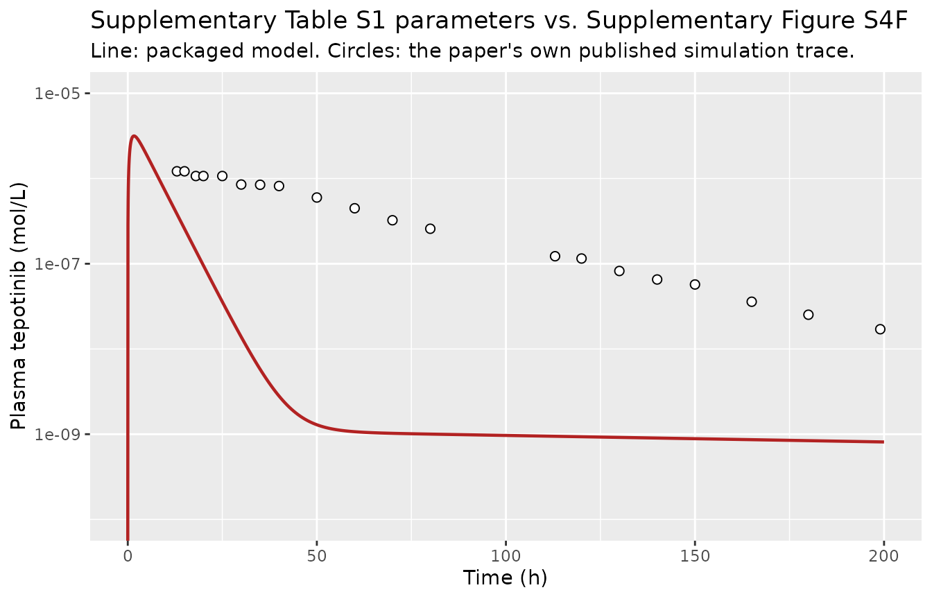

The packaged model against Supplementary Figure S4F of Hu 2025 (tepotinib 500 mg single oral dose, human). Open circles are the published simulation trace; the line is the model built from the parameters printed in the same paper’s Supplementary Table S1.

Side by side as NCA parameters, over the 13-199 h window where the figure is readable. Both sides are computed with PKNCA over the identical interval and the identical times, so the comparison is like for like. Every row is expected to be flagged; that is the finding, not a defect in the comparison.

window_nca <- function(dat, label) {
  conc <- dat |>
    dplyr::transmute(id = 1L, treatment = label, time,
                     Cc = conc_M * 1000 * MW_TEPOTINIB)   # mol/L -> ug/mL
  PKNCA::pk.nca(PKNCA::PKNCAdata(
    PKNCA::PKNCAconc(conc, Cc ~ time | treatment + id),
    PKNCA::PKNCAdose(
      tibble::tibble(id = 1L, treatment = label, time = 0, amt = DOSE_MG),
      amt ~ time | treatment + id
    ),
    intervals = data.frame(start = 13, end = 199,
                           cmax = TRUE, auclast = TRUE, half.life = TRUE)
  ))
}

ref_nca <- window_nca(figS4F, "500 mg single oral dose")
sim_win <- window_nca(
  tibble::tibble(time = cmp_pts$time, conc_M = cmp_pts$predicted),
  "500 mg single oral dose"
)

cmp <- nlmixr2lib::ncaComparisonTable(
  simulated     = sim_win,
  reference     = ref_nca,
  by            = "treatment",
  params        = c("cmax", "auclast", "half.life"),
  units         = c(cmax = "ug/mL", auclast = "ug*h/mL", half.life = "h"),
  tolerance_pct = 20
)

knitr::kable(cmp, caption = paste(
  "Packaged model (printed Supplementary Table S1 parameters) vs. the paper's",
  "own Supplementary Figure S4F, over 13-199 h.",
  "* differs from the reference by more than 20%."
))

Packaged model (printed Supplementary Table S1 parameters) vs. the paper’s own Supplementary Figure S4F, over 13-199 h. * differs from the reference by more than 20%.
NCA parameter	treatment	Reference	Simulated	% diff
Cmax (ug/mL)	500 mg single oral dose	0.599	0.189	-68.4%*
AUClast (ug*h/mL)	500 mg single oral dose	27.7	1.03	-96.3%*
t½ (h)	500 mg single oral dose	29.2	392	+1242.3%*

# The "% diff" column is a formatted string, and every row here also carries
# the out-of-tolerance flag, so the entries look like "-96.3%*". Strip the sign,
# the percent sign AND the asterisk -- a bare as.numeric() would coerce every
# entry to NA and make the assertion vacuously true.
pct <- as.numeric(gsub("[+%*]", "", cmp[["% diff"]]))
labels  <- cmp[["NCA parameter"]]
is_auc  <- grepl("^AUClast", labels)
is_thalf <- grepl("^t", labels)   # "t1/2 (h)", however PKNCA spells the label

stopifnot(
  length(pct) == 3L,
  !anyNA(pct),
  sum(is_auc) == 1L, sum(is_thalf) == 1L,
  # Every row carries the out-of-tolerance flag, and the misses are an order of
  # magnitude past the 20% tolerance rather than marginal. This locks the
  # documented contradiction in place: exposure is far too low and the terminal
  # half-life far too long.
  all(grepl("\\*$", cmp[["% diff"]])),
  all(abs(pct) > 50),
  pct[is_auc] < -90,
  pct[is_thalf] > 1000
)
round(pct, 1)
#> [1]  -68.4  -96.3 1242.3

Assumptions and deviations

The packaged model does not reproduce the paper’s own tepotinib figure, and ships anyway. This is a deliberate, operator-ratified decision for this extraction, and it is the single most important thing to know before using the model. The choice was between transcribing what Supplementary Table S1 prints (which fails against Supplementary Figure S4F) and substituting disposition parameters obtained by fitting a curve to that figure (which reproduces it, but puts two extractor-invented, load-bearing numbers into a packaged model in place of printed, source-attributed ones). Source fidelity was preferred: the printed values ship as printed, and the contradiction is documented here rather than repaired. The library has precedent for fitting a figure to fill a reporting gap – Beredaki_2023_micafungin_clsi and Zhu_2024_borneol_rat_pbpk both do – but none for overriding printed, source-attributed values with an extractor-side fit.

For the record, and to give a future reader something to check an author reply against: a one-compartment model with ka held at the printed 0.2 1/h tracks the Figure S4F trace closely when CL/F is near 15 L/h and V/F near 610 L. Those numbers are not in the packaged model and should not be treated as the paper’s. An author query has been filed asking for the disposition parameters actually used to produce Supplementary Figure S4F; if the authors reply, this model will be revised.

Practically: use this model to study the QSP framework as published. Do not use it to predict tepotinib exposure without first supplying disposition parameters of your own.

Reaction v69 is encoded in its mass-conserving form. Supplementary Table S1 prints the tepotinib distribution flux as Q/Vc*tepo_c*Vc/Vp_tepo-Q/Vp_tepo*tepo_p*Vp_tepo/Vc, which reduces to Q*tepo_c/Vp_tepo - Q*tepo_p/Vc: the two volume divisors are transposed relative to the standard inter-compartmental flux, and total drug is not conserved. The standard form Q*(tepo_c/Vc - tepo_p/Vp_tepo) is encoded instead, on the grounds that a distribution flux which creates or destroys drug cannot be what the authors’ SimBiology model integrated. This correction is not the cause of the disagreement with Figure S4F – taking the printed flux literally fits that figure very much worse still.

Two compartments, not one. Supplementary Table S1’s footnote names tepotinib as the “two-compartment” clinical PK exemplar, reaction v69 is an inter-compartmental distribution flux, and the Species sheet carries a tepo_p peripheral species. Supplementary Figure S9, the topology schematic, draws tepotinib with a central compartment only. The reaction list is followed, per the standing convention that a printed equation outranks a schematic; this also has the property that all five printed parameters are used, whereas a one-compartment reading would require discarding Q and vp_tepo.

CL was derived from a printed rate constant. Reaction v68 applies kcl_tepo to the central amount, so it is an elimination rate constant, and the clearance the nlmixr2 convention stores is kcl_tepo * Vc = 1.32 x 34 = 44.88 L/h. This is an exact algebraic restatement of two printed values, not a new number; CL / Vc recovers kcl_tepo exactly. Flows and volumes are stored rather than micro-constants so that rxSolve()’s default useLinCmt rewrite cannot silently collapse the peripheral compartment (the structural check above asserts against the analytic beta root for exactly this reason).

Bioavailability. Reaction v67 absorbs the full administered amount, so no F is applied and the disposition parameters are apparent (F = 1) parameters. Johne 2020, the cited PK source, is not on disk for this extraction.

Dose basis. Supplementary Figure S4F’s legend says 500 mg. The Results section distinguishes a 500 mg tablet from its 450 mg active moiety for Figure 7B, so a 10% dose ambiguity exists; it is far too small to affect anything discussed above.

No variability. The paper reports no between-subject variance and no residual-error model for any PK module, so propSd is encoded fixed(0) and the model is a typical-value simulator. Users running stochastic simulations must supply their own magnitudes.

Scope – only the PK submodule is packaged. Supplementary Table S1 prints all 69 reaction rate laws of the QSP network, but seven quantities those rate laws consume are reported nowhere in any on-disk source (main text, all three sheets of Table1.xlsx, DataSheet1.pdf, or the Figure S9 topology diagram):

km_egf, the Michaelis constant in v36.
baseline_cell, the additive basal-proliferation term in v59.
ki_tram, trametinib MEK-inhibition potency in v14 (no trametinib PK parameters are given either, so the whole MEK-inhibitor arm is unparameterized).
nmeto, the Hill exponent in v31.
Initial conditions / total pool sizes for every conserved species (AKT, MEK, ERK and their _14EX / _METO replicates, ALK, ROS1, HGF, and the three tumour-cell states). These have no synthesis or degradation reaction, so their totals are free initial conditions that fully determine model behaviour; the Methods state only that species were run to steady state, which pins the phospho-forms but not the conserved totals.
The plasma-to-intracellular partition coefficients. The Methods say tumour exposure was “proportional to drug exposure in the plasma by using calibrated partition coefficients”, but no coefficient is tabulated and Table S1 contains no reaction linking a *_c central species to its intracellular counterpart – so the PK modules are structurally disconnected from the signalling module and cannot drive it.
No central volume for crizotinib, so an absolute mg dose cannot be mapped onto crizo_c.

Per the library’s PBPK/QSP sourcing rule these are not filled in from class-typical values, and the network half of the paper is deferred pending author correspondence. Table S1’s own footnote confirms that the disclosure is deliberately partial (“exemplar equations … were listed here”), with 12 of the 16 drugs’ mechanisms and 14 of 16 PK modules never disclosed.

Other transcription defects in Supplementary Table S1 (recorded, but not affecting the packaged model): the Species sheet’s flux column is written against an earlier reaction numbering in several rows (ERK | v17-v16 and ERK_P | v16-v17 reference v17, “Production of exon 14 c-MET”, when the ERK phosphorylation pair is v15/v16; MEK_14EX | v14-v22-v23 references the MET autophosphorylation reactions); v7 lists savol_CMET twice; and v54 spells the complex crizo_CEMT.