Crovalimab (Cosson 2025)
Source:vignettes/articles/Cosson_2025_crovalimab.Rmd
Cosson_2025_crovalimab.RmdModel and source
- Citation: Cosson V, Fu R, Kulasekararaj A, Nishimura JI, Panse J, Roth A, Scheinberg P, Tong H, Yoon SS, Beveridge L, Gotanda K, Jaminion F, Henrich A, Lundberg P, Shi D, Sreckovic S, Zhang Y, Zhang Z, Benkali K, Buatois S. Pharmacokinetic characterization and exposure-response relationship of crovalimab in the COMMODORE 1, 2 and 3 and COMPOSER trials of patients with paroxysmal nocturnal haemoglobinuria. Br J Clin Pharmacol. 2025;91(5):1479. doi:10.1111/bcp.16394
- Description: Two-compartment population PK model of crovalimab (anti-C5 recycling monoclonal antibody) with first-order subcutaneous absorption and logit-normal bioavailability, plus an exponentially decaying additional clearance in patients switching from another C5 inhibitor (transient drug-target-drug immune complexes), in healthy volunteers and patients with paroxysmal nocturnal haemoglobinuria from the COMPOSER and COMMODORE 1, 2 and 3 trials (Cosson 2025)
- Article: https://doi.org/10.1111/bcp.16394 (open access; PMC12035591)
- Supplement: Supporting Information file 1 of the article (NONMEM control stream, Supplemental Results covariate equations and Table S3 parameter estimates).
Crovalimab is a recycling anti-C5 monoclonal antibody given as a
single intravenous (IV) loading dose followed by subcutaneous (SC)
loading and every-4-week maintenance doses. The final population PK
model is a two-compartment model with first-order SC absorption and a
logit-normal bioavailability. Patients switching from eculizumab or
ravulizumab, which bind a different C5 epitope, form transient
drug-target-drug immune complexes with crovalimab; the model describes
their faster early elimination with an additional clearance
CLs that decays exponentially with time since the first
crovalimab dose.
The paper also reports graphical PK/PD (CH50, free C5, normalised LDH) and logistic exposure-safety analyses. Those are LOESS smooths and logistic fits whose coefficients are not printed (only Wald p-values are given in Figure 6 and Figure S6), so no PD or exposure-safety sub-model can be packaged.
Population
The analysis pooled 430 participants from four studies (Table S1): 9 healthy volunteers from COMPOSER Part 1, 210 patients with paroxysmal nocturnal haemoglobinuria (PNH) naive to complement inhibition and 211 PNH patients switching from standard-dose eculizumab, higher-than-approved-dose eculizumab (n = 10) or ravulizumab (n = 21). Across studies, age ranged from 13 to 85 years and body weight from 40.6 to 140 kg (Table 2: naive median 65.2 kg and 35.5 years; switch median 71.0 kg and 44.0 years). The Phase III regimen (Table 1) is weight-tiered: 1000 mg IV on day 1 (1500 mg at >= 100 kg), 340 mg SC on days 2, 8, 15 and 22, then 680 mg SC (1020 mg at >= 100 kg) on day 29 and every 4 weeks. Anti-drug antibodies with titres >= 10^4 occurred in 8.1% of the analysis population. Sex and race distributions are not reported.
The same information is available programmatically via
readModelDb("Cosson_2025_crovalimab")()$population.
Source trace
| Equation / parameter | Value | Source location |
|---|---|---|
lcl_exp_inf (CL) |
0.0791 L/day | Table S3 ‘CL’; Results text |
lcl_exp_component (CLs) |
0.0341 L/day | Table S3 ‘CLs’ |
lcl_exp_kdes (Kd) |
0.0144 1/day | Table S3 ‘Kd’ |
lvc (V2) |
3.23 L | Table S3 ‘V2’; Results text |
lq (Q) |
0.168 L/day | Table S3 ‘Q’ |
lvp (V3) |
2.32 L | Table S3 ‘V3’; Results text |
lka (Ka) |
0.126 1/day | Table S3 ‘Ka’ |
logitfdepot (F) |
logit(0.830) | Table S3 ‘F’; logit-normal form from control stream
F1
|
e_wt_cl |
0.75 (fixed) | Table S3 ‘WT on CL and Q’ (FIX); control stream
CLS = CLSP*CLWT
|
e_wt_vc |
0.683824 | Supplemental Results covariate equations (Table S3: 0.684) |
e_ada_cl_exp_inf |
0.247352 | Supplemental Results covariate equations (Table S3: 0.247) |
e_age_ka |
-0.459 | Table S3 ‘Age on Ka’; Supplemental Results equation |
| IIV CL, V2, Ka, F, V3, Q | 0.206, 0.224, 0.383, 1.16, 0.706, 0.584 (SD) | Table S3; variance = SD^2 |
propSd |
0.113 | Table S3 ‘Proportional RUV’ |
addSdIntensive / addSdSparse
|
1.01 / 14.4 ug/mL | Table S3 ‘Additive RUV rich / sparse sampling’ |
etaaddSd |
0.787 (SD) | Table S3 ‘IIV additive RUV’; control stream
THETA(9)*EXP(ETA(8))
|
cl = cl_exp_inf + cl_exp_component * exp(-cl_exp_kdes * t) |
n/a | Control stream $DES
(CLN + CLS*EXP(-KD*T))/V2
|
d/dt(depot), d/dt(central),
d/dt(peripheral1)
|
n/a | Control stream $DES (ADVAN6, 3 compartments) |
Residual Cc ~ add(addSd) + prop(propSd)
|
n/a | Control stream $ERROR
W = SQRT(PROP^2*IPRED^2 + ADD^2)
|
Table S3 labels the IIV and residual-variability magnitudes “CV” and
notes that their RSEs are on the approximate SD scale. The supplement
$OMEGA block (0.0418, 0.0496, 0.140, 1.39, 0.494, 0.336,
0.617) equals the squares of the Table S3 values to within the
difference between the listed initial estimates and the final estimates,
so each value is an SD on the eta scale and the model uses its square as
the variance. The logit-scale SD of 1.16 on F could not be a log-normal
CV in any case.
Typical-value checks
The paper states several typical-value quantities that follow directly from the parameters. They are deterministic, so the checks are tight.
mod <- readModelDb("Cosson_2025_crovalimab")
ui <- rxode2::rxode(mod)
#> ℹ parameter labels from comments will be replaced by 'label()'
#> Warning: some etas defaulted to non-mu referenced, possible parsing error: etaaddSd
#> as a work-around try putting the mu-referenced expression on a simple line
th <- ui$theta

cl <- exp(th[["lcl_exp_inf"]])
vc <- exp(th[["lvc"]])
vp <- exp(th[["lvp"]])
q <- exp(th[["lq"]])

# Terminal half-life of the typical (75 kg, naive, ADA-negative) patient:
# the smaller root of the two-compartment characteristic polynomial.
k10 <- cl / vc
k12 <- q / vc
k21 <- q / vp
s <- k10 + k12 + k21
beta <- (s - sqrt(s^2 - 4 * k10 * k21)) / 2
thalf <- log(2) / beta

# Weight effects relative to 75 kg (Results: +35.1% / +31.6% at 112 kg,
# -29.6% / -27.4% at 47 kg for clearances / volumes).
wt_eff <- data.frame(
  WT = c(112, 112, 47, 47),
  parameter = c("clearances", "volumes", "clearances", "volumes"),
  published_pct = c(35.1, 31.6, -29.6, -27.4)
) |>
  mutate(
    exponent = ifelse(parameter == "clearances", th[["e_wt_cl"]], th[["e_wt_vc"]]),
    model_pct = 100 * ((WT / 75)^exponent - 1)
  )

# Switch clearance after 12 weeks as a share of total clearance
# (Discussion: 11.4%).
cls_84 <- exp(th[["lcl_exp_component"]]) * exp(-exp(th[["lcl_exp_kdes"]]) * 84)
share_84 <- 100 * cls_84 / (cl + cls_84)

knitr::kable(
  data.frame(
    Quantity = c("Terminal half-life (days)", "CLs share of total CL at week 12 (%)"),
    Published = c(53.1, 11.4),
    Model = signif(c(thalf, share_84), 3)
  ),
  caption = "Typical-value quantities stated in Cosson 2025 (Results and Discussion)."
)| Quantity | Published | Model |
|---|---|---|
| Terminal half-life (days) | 53.1 | 53.1 |
| CLs share of total CL at week 12 (%) | 11.4 | 11.4 |
knitr::kable(wt_eff, digits = c(0, 0, 1, 4, 1), caption = "Body-weight effects relative to 75 kg (Results).")| WT | parameter | published_pct | exponent | model_pct |
|---|---|---|---|---|
| 112 | clearances | 35.1 | 0.7500 | 35.1 |
| 112 | volumes | 31.6 | 0.6838 | 31.6 |
| 47 | clearances | -29.6 | 0.7500 | -29.6 |
| 47 | volumes | -27.4 | 0.6838 | -27.4 |
stopifnot(
  abs(thalf - 53.1) < 0.5,
  abs(share_84 - 11.4) < 0.1,
  all(abs(wt_eff$model_pct - wt_eff$published_pct) < 0.1)
)
Typical steady-state trough with and without ADA
The Results report a steady-state trough of 219 ug/mL without ADA and 166 ug/mL with ADA titres >= 10^4 “in a typical patient”. The patient is taken here as the covariate reference (75 kg, 36 years, naive, ADA-negative or ADA titre >= 10^4) on the < 100 kg regimen, with the trough read just before the day-365 maintenance dose.
# Phase III regimen (Table 1). Day 1 = time 0. The IV infusion duration is not
# stated in the paper; a 1-hour infusion is assumed (rate in mg/day).
regimen_events <- function(id, WT) {
  hi <- WT >= 100
  iv <- if (hi) 1500 else 1000
  maint <- if (hi) 1020 else 680
  sc_times <- c(1, 7, 14, 21, seq(28, 336, by = 28))
  sc_amts <- c(rep(340, 4), rep(maint, length(seq(28, 336, by = 28))))
  bind_rows(
    data.frame(id = id, time = 0, amt = iv, rate = iv * 24, evid = 1, cmt = "central"),
    data.frame(id = id, time = sc_times, amt = sc_amts, rate = 0, evid = 1, cmt = "depot")
  )
}
obs_times <- sort(unique(c(seq(0, 336, by = 1), seq(336, 364, by = 0.25))))
obs_rows <- function(id) {
  data.frame(id = id, time = obs_times, amt = 0, rate = 0, evid = 0, cmt = "central")
}
typ_events <- bind_rows(
  regimen_events(1L, 75), obs_rows(1L),
  regimen_events(2L, 75), obs_rows(2L)
) |>
  mutate(
    WT = 75, AGE = 36,
    ADA_TITER = ifelse(id == 2L, 1e4, 0),
    CONMED_ECULIZUMAB_BL = 0, CONMED_RAVULIZUMAB_BL = 0,
    SAMPLE_INTENSIVE = 0
  ) |>
  arrange(id, time, desc(evid))

typ <- rxode2::rxSolve(rxode2::zeroRe(mod), events = typ_events, returnType = "data.frame")
#> ℹ parameter labels from comments will be replaced by 'label()'
#> Warning: some etas defaulted to non-mu referenced, possible parsing error: etaaddSd
#> as a work-around try putting the mu-referenced expression on a simple line
#> Warning: some etas defaulted to non-mu referenced, possible parsing error: etaaddSd
#> as a work-around try putting the mu-referenced expression on a simple line
#> ℹ omega/sigma items treated as zero: 'etalcl_exp_inf', 'etalvc', 'etalka', 'etalogitfdepot', 'etalvp', 'etalq', 'etaaddSd'
#> Warning: multi-subject simulation without without 'omega'
trough <- typ |>
  filter(time == 364) |>
  transmute(ADA = ifelse(id == 2L, "ADA titre >= 10^4", "No ADA"), model = Cc) |>
  mutate(published = ifelse(ADA == "No ADA", 219, 166), pct_diff = 100 * (model / published - 1))
knitr::kable(trough, digits = 1, caption = "Typical steady-state trough (ug/mL), Results section.")| ADA | model | published | pct_diff |
|---|---|---|---|
| No ADA | 219.8 | 219 | 0.4 |
| ADA titre >= 10^4 | 169.7 | 166 | 2.2 |
Virtual cohort
Observed data are not public. The cohorts below approximate Table 2:
body weight log-normal with the published mean and SD, truncated to the
observed range; age normal with the published mean and SD, truncated to
the observed range. Each cohort has 200 patients. Naive patients carry
no switch indicator; switch patients are coded as switching from
eculizumab (CONMED_ECULIZUMAB_BL = 1; the model treats
ravulizumab identically). All patients are ADA-negative and observations
are on the sparse-sampling stratum.
rxode2::rxSetSeed(20251)
set.seed(20251)

rtrunc_lnorm <- function(n, mean, sd, lo, hi) {
  s2 <- log(1 + (sd / mean)^2)
  mu <- log(mean) - s2 / 2
  out <- numeric(0)
  while (length(out) < n) {
    x <- rlnorm(n, mu, sqrt(s2))
    out <- c(out, x[x >= lo & x <= hi])
  }
  out[seq_len(n)]
}
rtrunc_norm <- function(n, mean, sd, lo, hi) {
  out <- numeric(0)
  while (length(out) < n) {
    x <- rnorm(n, mean, sd)
    out <- c(out, x[x >= lo & x <= hi])
  }
  out[seq_len(n)]
}

make_cohort <- function(n, cohort, wt_mean, wt_sd, wt_lo, wt_hi,
                        age_mean, age_sd, age_lo, age_hi, switch, id_offset) {
  subj <- data.frame(
    id = id_offset + seq_len(n),
    WT = rtrunc_lnorm(n, wt_mean, wt_sd, wt_lo, wt_hi),
    AGE = rtrunc_norm(n, age_mean, age_sd, age_lo, age_hi)
  )
  ev <- bind_rows(lapply(seq_len(n), function(i) {
    bind_rows(regimen_events(subj$id[i], subj$WT[i]), obs_rows(subj$id[i]))
  }))
  ev |>
    left_join(subj, by = "id") |>
    mutate(
      cohort = cohort,
      ADA_TITER = 0,
      CONMED_ECULIZUMAB_BL = switch,
      CONMED_RAVULIZUMAB_BL = 0,
      SAMPLE_INTENSIVE = 0
    )
}

events <- bind_rows(
  make_cohort(200, "Naive", 67.9, 15.0, 42.0, 140, 39.2, 15.1, 13, 76, 0, id_offset = 0L),
  make_cohort(200, "Switch", 72.9, 17.9, 40.6, 132, 45.0, 15.3, 16, 85, 1, id_offset = 200L)
) |>
  arrange(id, time, desc(evid))
stopifnot(!anyDuplicated(unique(events[, c("id", "time", "evid")])))
Simulation
sim <- rxode2::rxSolve(mod, events = events, keep = c("cohort", "WT"), returnType = "data.frame")
#> ℹ parameter labels from comments will be replaced by 'label()'
#> Warning: some etas defaulted to non-mu referenced, possible parsing error: etaaddSd
#> as a work-around try putting the mu-referenced expression on a simple line
Replicate published figures
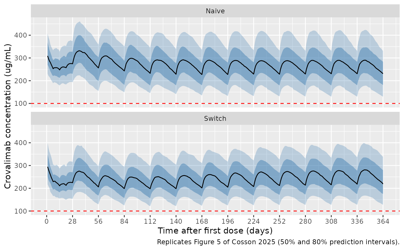
Figure 5: simulated concentration-time profiles
# Replicates Figure 5 of Cosson 2025: median with 50% and 80% prediction
# intervals for naive (A) and switch (B) patients on the recommended regimen.
sim |>
  filter(time >= 1 / 24) |>
  group_by(cohort, time) |>
  summarise(
    p10 = quantile(Cc, 0.10), p25 = quantile(Cc, 0.25),
    p50 = median(Cc),
    p75 = quantile(Cc, 0.75), p90 = quantile(Cc, 0.90),
    .groups = "drop"
  ) |>
  ggplot(aes(time, p50)) +
  geom_ribbon(aes(ymin = p10, ymax = p90), fill = "steelblue", alpha = 0.3) +
  geom_ribbon(aes(ymin = p25, ymax = p75), fill = "steelblue", alpha = 0.5) +
  geom_line() +
  geom_hline(yintercept = 100, linetype = "dashed", colour = "red") +
  facet_wrap(~cohort, ncol = 1) +
  scale_x_continuous(breaks = seq(0, 364, by = 28)) +
  labs(
    x = "Time after first dose (days)", y = "Crovalimab concentration (ug/mL)",
    caption = "Replicates Figure 5 of Cosson 2025 (50% and 80% prediction intervals)."
  )
Proportion of patients above 100 ug/mL throughout treatment
The Results report that 92.8% of naive and 91.4% of switch patients were predicted to stay above 100 ug/mL over the whole treatment course.
above <- sim |>
  filter(time >= 1) |>
  group_by(cohort, id) |>
  summarise(always_above = all(Cc > 100), .groups = "drop") |>
  group_by(cohort) |>
  summarise(model_pct = 100 * mean(always_above), .groups = "drop") |>
  mutate(published_pct = c(Naive = 92.8, Switch = 91.4)[cohort])
knitr::kable(above, digits = 1, caption = "Patients with concentrations above 100 ug/mL from day 2 to day 365 (%).")| cohort | model_pct | published_pct |
|---|---|---|
| Naive | 97 | 92.8 |
| Switch | 95 | 91.4 |
# With 200 patients per cohort the binomial SE is about 2 percentage points;
# the cohort covariates are approximations of Table 2. Across three cohort
# draws the differences ranged from -1.9 to +4.7 points. A mis-transcribed
# clearance, volume or bioavailability moves this share by tens of points.
stopifnot(all(abs(above$model_pct - above$published_pct) < 10))
PKNCA validation
NCA over the last maintenance interval (days 337 to 365, i.e. time 336 to 364), grouped by cohort. The paper reports a median steady-state Tmax of 8.27 days after SC administration across the Phase III studies (pooled over naive and switch patients). Steady-state Cmax and trough are digitised by the maintainers from the median curves of Figure 5 (approximately 270 and 215 ug/mL for naive patients, 255 and 203 ug/mL for switch patients).
sim_nca <- sim |>
  filter(!is.na(Cc), time >= 336, time <= 364) |>
  select(id, time, Cc, cohort)

conc_obj <- PKNCA::PKNCAconc(sim_nca, Cc ~ time | cohort + id)
dose_df <- events |>
  filter(evid == 1, time == 336) |>
  select(id, time, amt, cohort)
dose_obj <- PKNCA::PKNCAdose(dose_df, amt ~ time | cohort + id)
intervals <- data.frame(start = 336, end = 364, cmax = TRUE, tmax = TRUE, cmin = TRUE, auclast = TRUE)
nca_res <- PKNCA::pk.nca(PKNCA::PKNCAdata(conc_obj, dose_obj, intervals = intervals))

# PKNCA reports tmax relative to the interval start (the day-337 dose).
nca_long <- as.data.frame(nca_res$result)

published <- tibble::tribble(
  ~cohort, ~cmax, ~tmax, ~cmin,
  "Naive", 270, 8.27, 215,
  "Switch", 255, 8.27, 203
)
cmp <- nlmixr2lib::ncaComparisonTable(
  simulated = nca_long,
  reference = published,
  by = "cohort",
  params = c("cmax", "tmax", "cmin"),
  units = c(cmax = "ug/mL", tmax = "day", cmin = "ug/mL"),
  tolerance_pct = 20
)
knitr::kable(cmp, caption = "Simulated vs. published steady-state NCA (medians). * differs from reference by >20%.")| NCA parameter | cohort | Reference | Simulated | % diff |
|---|---|---|---|---|
| Cmax (ug/mL) | Naive | 270 | 291 | +7.9% |
| Cmax (ug/mL) | Switch | 255 | 281 | +10.4% |
| Cmin (ug/mL) | Naive | 215 | 231 | +7.2% |
| Cmin (ug/mL) | Switch | 203 | 218 | +7.4% |
| Tmax (day) | Naive | 8.27 | 8.38 | +1.3% |
| Tmax (day) | Switch | 8.27 | 8.75 | +5.8% |
sim_med <- nca_long |>
  filter(PPTESTCD %in% c("cmax", "cmin")) |>
  group_by(cohort, PPTESTCD) |>
  summarise(sim = median(PPORRES), .groups = "drop") |>
  left_join(
    tidyr::pivot_longer(published, c(cmax, cmin), names_to = "PPTESTCD", values_to = "ref"),
    by = c("cohort", "PPTESTCD")
  )
# Medians of 200 patients against values digitised from a published median
# curve. Across three cohort draws the four ratios ranged from +3% to +13%
# (mean +7% to +8%), so the centre is gated tightly and each row loosely.
# A dose, volume or bioavailability error moves all four by >= 20%.
ratio <- sim_med$sim / sim_med$ref - 1
stopifnot(
  abs(mean(ratio)) < 0.15,
  all(abs(ratio) < 0.25)
)

# Median steady-state Tmax against the published 8.27 days. The typical
# patient peaks at 8.25 days; the cohort median sits on the 0.25-day grid.
# An absorption rate off by a factor of 2 moves Tmax by several days.
tmax_med <- nca_long |>
  filter(PPTESTCD == "tmax") |>
  group_by(cohort) |>
  summarise(tmax = median(PPORRES), .groups = "drop")
stopifnot(all(abs(tmax_med$tmax - 8.27) < 1.5))
Simulated steady-state median Cmax and trough sit a few percent to about 13% above the values read from Figure 5, depending on the cohort draw, and the share of patients staying above 100 ug/mL is usually a few points above the published 92.8% and 91.4%. Both differences point the same way and are consistent with the simulated cohorts being entirely ADA-negative (8.1% of the analysis population had titres >= 10^4, which raise CL by 24.7%) and with the Table 2 marginals standing in for the paper’s representative population. The typical-patient trough, which removes the cohort entirely, matches the published value to within 0.5%.
Assumptions and deviations
- The IV infusion duration is not reported; a 1-hour infusion is assumed. With a 53-day terminal half-life the choice has no visible effect beyond the first hours.
- Time in the switch clearance
exp(-Kd * t)is time since the first crovalimab dose (the NONMEM$DEST). Simulations must start the event table at the first crovalimab dose. - The source switch-status column
SWITCHcodes three prior agents (standard-dose eculizumab, high-dose eculizumab, ravulizumab) that the paper found to act alike on CLs. It is represented here by two baseline indicators,CONMED_ECULIZUMAB_BLandCONMED_RAVULIZUMAB_BL, and the model uses their maximum. - The ADA effect uses a three-group titre categorisation in the source
(
ADA3T3G, groups 2 and 3 described as “medium or high titer ADA”). The Results identify these as titres >= 10^4, so the model applies the 24.7% CL increase whenADA_TITER >= 10000. - IIV on CLs, Kd and the proportional residual error is fixed to 0 in the source control stream and is omitted.
- Residual error: the source uses a rich-sampling additive SD
(COMPOSER Part 1 healthy volunteers and study YO42311) and a
sparse-sampling additive SD with between-subject variability on its
magnitude, selected here by
SAMPLE_INTENSIVE. - Virtual cohorts approximate Table 2 marginals only. Sex and race are not reported and are not model covariates. All simulated patients are ADA-negative because the paper does not say whether its Figure 5 population included ADA-positive patients.
- The paper’s PK/PD (CH50, free C5, LDH) and exposure-safety analyses are graphical or logistic regressions with unreported coefficients and are not packaged.
- No erratum or correction notice was found for the article (Europe PMC search, 2026-11-04).