Model and source
- Citation: Yu M, Liu S, Wu X, Wang H. Population pharmacokinetic modeling of ilaprazole in healthy subjects and patients with duodenal ulcer in China. Front Pharmacol. 2024 Jan 10;14:1306222. doi:10.3389/fphar.2023.1306222.
- Description: Two-compartment population PK model with first-order elimination for ilaprazole, a proton-pump inhibitor, after 0.75 h intravenous infusion in Chinese healthy subjects and patients with duodenal ulcer (Yu 2024). Pooled analysis of 1,560 plasma concentrations from 58 subjects across four phase I studies (healthy) and one phase IIa study (duodenal ulcer), fit in Phoenix NLME 8.3 by FOCE-ELS. Female sex lowers clearance (exp(-0.213)) and duodenal-ulcer disease status raises both clearance (exp(0.290)) and peripheral volume (exp(0.356)); peripheral volume additionally scales with body weight by a power of 1.545 around a 60.6 kg median. Typical values are for a healthy male at 60.6 kg. Inter-individual variability on the inter-compartmental clearance (CLp) was fixed in the final model because of 84% eta-shrinkage and no numeric variance was reported, so it is encoded as fixed(0).
- Article: https://doi.org/10.3389/fphar.2023.1306222
- Supplementary material: https://www.frontiersin.org/articles/10.3389/fphar.2023.1306222/full#supplementary-material
Ilaprazole is a substituted-benzimidazole proton-pump inhibitor developed by Il-Yang Pharmacy (Seoul) and Livzon Pharmaceutical (Zhuhai). Unlike the first- and second-generation proton-pump inhibitors, ilaprazole is metabolised principally by CYP3A4/5 rather than CYP2C19, so its disposition is not affected by CYP2C19 genetic polymorphism; its half-life (4.7-5.3 h) is also substantially longer than that of omeprazole, lansoprazole, or pantoprazole. Yu 2024 is the first population PK analysis of ilaprazole in a Chinese population.
Population
The model was built on 1,560 valid plasma concentrations from 58 Chinese subjects enrolled in five clinical trials of intravenous ilaprazole (Yu 2024 Tables 1 and 2): four phase I studies in healthy subjects (CTR20132848 single-dose 4x4 crossover, n = 16; CTR20140147 multiple-dose, n = 10; CTR20150686 high-dose, n = 10; CTR20150685 loading-dose, n = 12) and one phase IIa study in patients with duodenal ulcer (CTR20132846, n = 10). Patients were required to have an ulcer diameter <= 15 mm with no combined ulcer bleeding, and, by the trial exclusion criteria, none had a history of smoking or drinking.
Pooled baseline characteristics (Table 2, “Total” column) were: median age 25 years (IQR 23-31; the duodenal-ulcer cohort was older at a median of 46 years), median height 168 cm (IQR 160.5-172.3), median weight 60.6 kg (IQR 55.8-65.1), median BMI 21.6 kg/m^2 (IQR 20.8-22.7), and median Cockcroft-Gault creatinine clearance 118.1 mL/min (IQR 98.2-124.1). 28 of 58 subjects (48.3%) were female. Doses were 5, 10, 20, and 30 mg, each given as an intravenous infusion over 0.75 h; the multiple-dose regimens used a 20 mg loading dose on day 1 followed by 10 mg maintenance doses on days 2-3. The bioanalytical assay (UPLC-MS/MS) was linear over 1-1,000 ng/mL with a 1 ng/mL lower limit of quantification; 5 below-limit-of-quantification and 7 not-detected samples were excluded.
The same information is available programmatically via the model’s
population metadata
(readModelDb("Yu_2024_ilaprazole")()$population).
Source trace
The per-parameter origin is recorded as an in-file comment next to
each ini() entry in
inst/modeldb/specificDrugs/Yu_2024_ilaprazole.R. The table
below collects them in one place for review.
| Equation / parameter | Value | Source location |
|---|---|---|
| Two-compartment structure, first-order elimination | n/a | Yu 2024 Section 3.2 (dOFV = 929.103 vs the
one-compartment model); Supplementary Figures S1-S2 |
Exponential IIV model P_ik = P_popk * exp(eta_ik)
|
n/a | Yu 2024 Eq. 1 |
Continuous-covariate power form
P = P_pop * (COVR_i / COVR_median)^theta
|
n/a | Yu 2024 Eq. 5 |
Categorical-covariate exponential form
P = P_pop * exp(theta * COVR_i)
|
n/a | Yu 2024 Eq. 6 |
V = V * exp(eta_V) |
n/a | Yu 2024 Eq. 7 |
CL = CL * exp(-0.213*Sex) * exp(0.29*Disease status) * exp(eta_CL) |
n/a | Yu 2024 Eq. 8 |
Vp = Vp * (Weight/60.6)^1.545 * exp(0.356*Disease status) * exp(eta_Vp) |
n/a | Yu 2024 Eq. 9 |
lvc (V) |
6.795 L | Table 3, “Typical value parameter of population” (RSE 5.230%, 95% CI 6.098-7.492) |
lcl (CL) |
3.394 L/h (healthy male) | Table 3 (RSE 3.225%, 95% CI 3.180-3.609) |
lvp (Vp) |
5.544 L (healthy, 60.6 kg) | Table 3 (RSE 7.182%, 95% CI 4.763-6.326) |
lq (CLp) |
13.086 L/h | Table 3 (RSE 16.896%, 95% CI 8.749-17.423) |
e_sexf_cl |
-0.213 | Table 3 “Sex effect on CL (Sex = 1)” and Eq. 8 (RSE -23.398%, 95% CI -0.311 to -0.115) |
e_dis_duod_ulcer_cl |
0.290 | Table 3 “Disease status effect on CL (Disease status = 1)” and Eq. 8 (RSE 23.751%, 95% CI 0.155-0.425) |
e_dis_duod_ulcer_vp |
0.356 | Table 3 “Disease status effect on Vp (Disease status = 1)” and Eq. 9 (RSE 14.707%, 95% CI 0.253-0.459) |
e_wt_vp |
1.545 | Table 3 “WT effect on Vp” and Eq. 9 (RSE 13.714%, 95% CI 1.129-1.960); median weight 60.6 kg |
etalvc (omega^2 V) |
0.013 | Table 3 “inter-individual variability” (RSE 31.284%, shrinkage 34.0%) |
etalvp (omega^2 Vp) |
0.032 | Table 3 (RSE 21.763%, shrinkage 1.82%) |
etalcl (omega^2 CL) |
0.059 | Table 3 (RSE 25.051%, shrinkage 24.4%) |
etalq (omega^2 CLp) |
fixed(0) |
Table 3 row reported only as “Fixed”; Section 3.2 (“CLp was fixed due to its high eta-shrinkage (84%)”) |
propSd (sigma_mult) |
0.184 | Table 3 “Residual variability” (RSE 9.131%, 95% CI 0.151-0.217) |
| Infusion duration 0.75 h | n/a | Yu 2024 Table 1 footnote (“In all of the above studies, the duration of intravenous infusion was 0.75 h”) |
| Median weight 60.6 kg (Vp normalisation) | n/a | Yu 2024 Eq. 9 and Table 2 “Total” column |
Covariate encoding
Yu 2024 codes its Disease status covariate as 1
= duodenal ulcer with the pooled healthy cohort as reference
(Table 3 footnote). That maps 1:1 onto the canonical covariate
DIS_DUOD_ULCER, so every Table 3 estimate is carried into
ini() verbatim – no sign flip and no re-baselining of the
typical values. Likewise the paper’s Sex is already coded 1
= female, matching canonical SEXF directly.
DIS_DUOD_ULCER was added to
inst/references/covariate-columns.md as part of this
extraction. It follows the established DIS_UC /
DIS_PSORIASIS / DIS_HAE pattern of
specific-disease-vs-non-disease cohort indicators, and is deliberately
distinct from ENDO_ULCER, which scores mucosal-ulcer
activity within an inflammatory-bowel-disease cohort – peptic
ulcer disease is a non-IBD upper-GI condition.
The typical values the model returns at the reference state are therefore exactly the paper’s Table 3 numbers:
c(
  CL_healthy_male = exp(log(3.394)),                  # Table 3: 3.394 L/h
  CL_ulcer_male   = exp(log(3.394) + 0.290),          # Eq. 8 disease effect
  CL_healthy_fem  = exp(log(3.394) - 0.213),          # Eq. 8 sex effect
  Vp_healthy      = exp(log(5.544)),                  # Table 3: 5.544 L
  Vp_ulcer        = exp(log(5.544) + 0.356)           # Eq. 9 disease effect
)
#> CL_healthy_male   CL_ulcer_male  CL_healthy_fem      Vp_healthy        Vp_ulcer
#>        3.394000        4.535835        2.742882        5.544000        7.914656
Virtual cohort
The original observed concentrations are not publicly available. Two virtual populations are built below.
scenarios is a deterministic (typical-value) covariate
grid used to reproduce the covariate-effect simulation of Yu 2024
Section 3.3 / Figure 3: a single 20 mg intravenous infusion over
0.75 h, evaluated at the reference state and at each covariate
perturbation in turn.
set.seed(20240110)

INFUSION_DUR <- 0.75   # h; Yu 2024 Table 1 footnote
DOSE_MG      <- 20     # mg; Yu 2024 Section 3.3 simulation dose
WT_MEDIAN    <- 60.6   # kg; Yu 2024 Eq. 9 normalisation constant

# Dense early grid to resolve the end-of-infusion peak, then out to 24 h
# (the last sampling time in every contributing study, i.e. AUC0-t = AUC0-24).
obs_times <- sort(unique(c(seq(0, 2, by = 0.05), seq(2, 24, by = 0.25))))

make_arm <- function(label, sexf, dis_duod_ulcer, wt, id) {
  ev <- rxode2::et(amt = DOSE_MG, dur = INFUSION_DUR, cmt = "central")
  ev <- rxode2::et(ev, obs_times, cmt = "central")
  out <- as.data.frame(ev)
  out$id             <- id
  out$scenario       <- label
  out$SEXF           <- sexf
  out$DIS_DUOD_ULCER <- dis_duod_ulcer
  out$WT             <- wt
  out
}

# SEXF: 1 = female. DIS_DUOD_ULCER: 1 = duodenal-ulcer patient, 0 = healthy.
scenarios <- dplyr::bind_rows(
  make_arm("Healthy male, 60.6 kg (reference)", 0, 0, WT_MEDIAN, 1L),
  make_arm("Healthy female, 60.6 kg",           1, 0, WT_MEDIAN, 2L),
  make_arm("Duodenal ulcer male, 60.6 kg",      0, 1, WT_MEDIAN, 3L),
  make_arm("Healthy male, 45 kg",               0, 0, 45,        4L),
  make_arm("Healthy male, 85 kg",               0, 0, 85,        5L)
)

# Guard against silently-collapsed subjects (duplicate id/time/evid keys).
stopifnot(!anyDuplicated(scenarios[, c("id", "time", "evid")]))
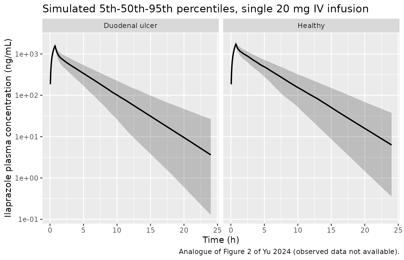
cohort is a stochastic virtual population of 200 healthy
subjects and 200 duodenal-ulcer patients, with covariates drawn to match
the Table 2 marginal distributions. It is used for the
concentration-time prediction intervals.
N_PER_ARM <- 200   # cohort cap: never more than 200 participants per arm

make_pop <- function(label, dis_duod_ulcer, n, id_offset, female_pct, wt_median, wt_sd) {
  covs <- tibble::tibble(
    id             = id_offset + seq_len(n),
    scenario       = label,
    DIS_DUOD_ULCER = dis_duod_ulcer,
    SEXF           = as.numeric(seq_len(n) <= round(n * female_pct)),
    WT             = pmax(40, rnorm(n, mean = wt_median, sd = wt_sd))
  )
  purrr_rows <- lapply(seq_len(nrow(covs)), function(i) {
    ev  <- rxode2::et(amt = DOSE_MG, dur = INFUSION_DUR, cmt = "central")
    ev  <- rxode2::et(ev, obs_times, cmt = "central")
    out <- as.data.frame(ev)
    out$id          <- covs$id[i]
    out$scenario    <- covs$scenario[i]
    out$SEXF        <- covs$SEXF[i]
    out$DIS_DUOD_ULCER <- covs$DIS_DUOD_ULCER[i]
    out$WT          <- covs$WT[i]
    out
  })
  dplyr::bind_rows(purrr_rows)
}

# Table 2: 48.3% female overall; healthy-study female fraction 50%, duodenal
# ulcer study 40%. Weight SD approximated from the reported IQR
# (IQR 55.8-65.1 kg => SD ~ IQR / 1.349 ~ 6.9 kg).
cohort <- dplyr::bind_rows(
  make_pop("Healthy",        0, N_PER_ARM,    0L, 0.50, 60.6, 6.9),
  make_pop("Duodenal ulcer", 1, N_PER_ARM, 1000L, 0.40, 63.0, 6.9)
)
Simulation
mod <- readModelDb("Yu_2024_ilaprazole")

# Typical-value (deterministic) run for the Figure 3 covariate comparison.
# `zeroRe()` alone is not sufficient: rxode2 re-samples etas when a stochastic
# solve has already run in the same session, so `omega = NA` is required to
# force a true typical-value solve.
mod_typical <- rxode2::zeroRe(mod)
#> ℹ parameter labels from comments will be replaced by 'label()'
sim_typical <- rxode2::rxSolve(
  mod_typical, events = scenarios, omega = NA, keep = "scenario"
)
#> Warning: multi-subject simulation without without 'omega'

# Stochastic run for the concentration-time prediction intervals.
sim_pop <- rxode2::rxSolve(mod, events = cohort, keep = "scenario")
#> ℹ parameter labels from comments will be replaced by 'label()'
#> ℹ omega/sigma items treated as zero: 'etalq'
Replicate published figures
Typical concentration-time profiles by covariate scenario
sim_typical |>
  dplyr::filter(time > 0) |>
  ggplot(aes(time, Cc, colour = scenario)) +
  geom_line(linewidth = 0.8) +
  scale_y_log10() +
  labs(
    x = "Time (h)", y = "Ilaprazole plasma concentration (ng/mL)",
    colour = NULL,
    title = "Typical profiles after a single 20 mg IV infusion over 0.75 h",
    caption = "Covariate scenarios underlying Figure 3 of Yu 2024."
  ) +
  theme(legend.position = "bottom") +
  guides(colour = guide_legend(nrow = 3))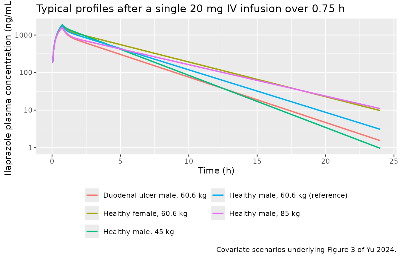
Prediction intervals (Figure 2 analogue)
Yu 2024 Figure 2 is a visual predictive check of the pooled analysis dataset. The observed concentrations are not available, so the panel below shows the model-simulated 5th, 50th, and 95th percentiles for the healthy and duodenal-ulcer virtual populations after a single 20 mg infusion.
sim_pop |>
  dplyr::filter(time > 0) |>
  dplyr::group_by(scenario, time) |>
  dplyr::summarise(
    Q05 = quantile(Cc, 0.05, na.rm = TRUE),
    Q50 = quantile(Cc, 0.50, na.rm = TRUE),
    Q95 = quantile(Cc, 0.95, na.rm = TRUE),
    .groups = "drop"
  ) |>
  ggplot(aes(time, Q50)) +
  geom_ribbon(aes(ymin = Q05, ymax = Q95), alpha = 0.25) +
  geom_line(linewidth = 0.8) +
  facet_wrap(~scenario) +
  scale_y_log10() +
  labs(
    x = "Time (h)", y = "Ilaprazole plasma concentration (ng/mL)",
    title = "Simulated 5th-50th-95th percentiles, single 20 mg IV infusion",
    caption = "Analogue of Figure 2 of Yu 2024 (observed data not available)."
  )
PKNCA validation
NCA is run on the typical-value scenarios, which is what Yu 2024
Figure 3 summarises. AUC0-t in the paper is the AUC to the
last sampling time, i.e. AUC0-24, so auclast
is computed over the 0-24 h interval; aucinf.obs and
half.life are reported alongside for completeness.
# Only `!is.na(Cc)` -- adding `time > 0` or `Cc > 0` would drop the time-zero
# row that PKNCA needs to anchor AUC0-t.
sim_nca <- sim_typical |>
  dplyr::filter(!is.na(Cc)) |>
  dplyr::select(id, time, Cc, scenario)

# Guarantee a time-zero record per subject (pre-dose concentration is 0 for an
# infusion that starts at t = 0).
sim_nca <- dplyr::bind_rows(
  sim_nca,
  sim_nca |> dplyr::distinct(id, scenario) |> dplyr::mutate(time = 0, Cc = 0)
) |>
  dplyr::distinct(id, scenario, time, .keep_all = TRUE) |>
  dplyr::arrange(id, scenario, time)

conc_obj <- PKNCA::PKNCAconc(
  sim_nca, Cc ~ time | scenario + id,
  concu = "ng/mL", timeu = "h"
)

dose_df <- scenarios |>
  dplyr::filter(evid != 0) |>
  dplyr::select(id, time, amt, scenario) |>
  dplyr::distinct()

dose_obj <- PKNCA::PKNCAdose(dose_df, amt ~ time | scenario + id, doseu = "mg")

intervals <- data.frame(
  start      = 0,
  end        = 24,
  cmax       = TRUE,
  tmax       = TRUE,
  auclast    = TRUE,
  aucinf.obs = TRUE,
  half.life  = TRUE
)

nca_res <- PKNCA::pk.nca(
  PKNCA::PKNCAdata(conc_obj, dose_obj, intervals = intervals)
)

nca_wide <- as.data.frame(nca_res) |>
  dplyr::select(scenario, PPTESTCD, PPORRES) |>
  tidyr::pivot_wider(names_from = PPTESTCD, values_from = PPORRES)

nca_wide |>
  dplyr::select(scenario, cmax, tmax, auclast, aucinf.obs, half.life) |>
  dplyr::mutate(dplyr::across(where(is.numeric), \(x) signif(x, 4))) |>
  dplyr::rename(
    "Scenario"            = scenario,
    "Cmax (ng/mL)"        = cmax,
    "Tmax (h)"            = tmax,
    "AUC0-24 (ng*h/mL)"   = auclast,
    "AUC0-inf (ng*h/mL)"  = aucinf.obs,
    "t1/2 (h)"            = half.life
  ) |>
  knitr::kable(
    caption = "Typical-value NCA after a single 20 mg IV infusion over 0.75 h.",
    align = c("l", "r", "r", "r", "r", "r")
)| Scenario | Cmax (ng/mL) | Tmax (h) | AUC0-24 (ng*h/mL) | AUC0-inf (ng*h/mL) | t1/2 (h) |
|---|---|---|---|---|---|
| Duodenal ulcer male, 60.6 kg | 1579 | 0.75 | 4404 | 4409 | 2.481 |
| Healthy female, 60.6 kg | 1790 | 0.75 | 7246 | 7291 | 3.244 |
| Healthy male, 45 kg | 1872 | 0.75 | 5890 | 5893 | 2.164 |
| Healthy male, 60.6 kg (reference) | 1742 | 0.75 | 5881 | 5893 | 2.649 |
| Healthy male, 85 kg | 1617 | 0.75 | 5836 | 5892 | 3.584 |
Terminal half-life is shorter than the literature value quoted in the paper
The typical healthy-male terminal half-life implied by the Table 3 parameter set is about 2.6 h, noticeably shorter than the 4.7-5.3 h that the Yu 2024 Introduction quotes for ilaprazole (citing Sachs 2006 and Shin 2014, which report oral ilaprazole). This is a property of the published parameters, not of the implementation – it can be derived in closed form from the two-compartment micro-constants without simulating anything:
cl <- 3.394; vc <- 6.795; vp <- 5.544; q <- 13.086   # Yu 2024 Table 3, healthy reference
kel <- cl / vc; k12 <- q / vc; k21 <- q / vp
s   <- kel + k12 + k21
beta <- 0.5 * (s - sqrt(s^2 - 4 * kel * k21))        # terminal disposition rate constant
c(
  `kel (1/h)`            = kel,
  `beta (1/h)`           = beta,
  `terminal t1/2 (h)`    = log(2) / beta,
  `Vss (L)`              = vc + vp,
  `MRT (h)`              = (vc + vp) / cl
)
#>         kel (1/h)        beta (1/h) terminal t1/2 (h)           Vss (L)
#>         0.4994849         0.2605384         2.6604415        12.3390000
#>           MRT (h)
#>         3.6355333
No tuning has been applied to close this gap. Two readings are
consistent with the source: the 4.7-5.3 h figure describes oral
ilaprazole in a different population, whereas this model was fit
exclusively to 0.75 h intravenous infusion data sampled only to 24 h;
and a terminal phase that contributes little to total exposure is poorly
identified by such a design. AUC0-inf and
AUC0-24 differ by only ~0.2% here, so the truncated
sampling window captures essentially all of the exposure regardless.
Comparison against published covariate effects
Yu 2024 does not tabulate absolute NCA values for its own dataset; Section 3.3 instead reports the percentage change in Cmax and AUC0-t produced by each significant covariate after a single 20 mg infusion (Figure 3). Those percentages are the validation target.
ref_row <- nca_wide |> dplyr::filter(scenario == "Healthy male, 60.6 kg (reference)")

pct <- function(scn, metric) {
  x <- nca_wide[[metric]][nca_wide$scenario == scn]
  100 * (x - ref_row[[metric]]) / ref_row[[metric]]
}

comparison <- tibble::tibble(
  Comparison = c(
    "Female vs male (healthy, 60.6 kg)",
    "Female vs male (healthy, 60.6 kg)",
    "Duodenal ulcer vs healthy (male, 60.6 kg)",
    "Duodenal ulcer vs healthy (male, 60.6 kg)",
    "Body weight 45 vs 85 kg (healthy male)",
    "Body weight 45 vs 85 kg (healthy male)"
  ),
  Parameter = c("Cmax", "AUC0-t", "Cmax", "AUC0-t", "Cmax", "AUC0-t"),
  Simulated = c(
    pct("Healthy female, 60.6 kg", "cmax"),
    pct("Healthy female, 60.6 kg", "auclast"),
    pct("Duodenal ulcer male, 60.6 kg", "cmax"),
    pct("Duodenal ulcer male, 60.6 kg", "auclast"),
    pct("Healthy male, 45 kg", "cmax") - pct("Healthy male, 85 kg", "cmax"),
    pct("Healthy male, 45 kg", "auclast") - pct("Healthy male, 85 kg", "auclast")
  ),
  Published = c(4.79, 24.73, -16.7, -26.92, NA, NA),
  `Published wording` = c(
    "4.79% higher in females", "24.73% higher in females",
    "16.7% decrease in patients", "26.92% decrease in patients",
    "affected Cmax by less than 25%", "mild impact on AUC0-t (~5%)"
  )
)

comparison |>
  dplyr::mutate(
    Simulated = signif(Simulated, 3),
    Difference = ifelse(is.na(Published), NA, signif(Simulated - Published, 3))
  ) |>
  dplyr::rename(
    "Simulated (%)"  = Simulated,
    "Published (%)"  = Published,
    "Difference (%)" = Difference
  ) |>
  knitr::kable(
    caption = "Simulated vs. published covariate effects on exposure (Yu 2024 Section 3.3 / Figure 3).",
    align = c("l", "l", "r", "r", "r", "l")
)| Comparison | Parameter | Simulated (%) | Published (%) | Published wording | Difference (%) |
|---|---|---|---|---|---|
| Female vs male (healthy, 60.6 kg) | Cmax | 2.760 | 4.79 | 4.79% higher in females | -2.03 |
| Female vs male (healthy, 60.6 kg) | AUC0-t | 23.200 | 24.73 | 24.73% higher in females | -1.53 |
| Duodenal ulcer vs healthy (male, 60.6 kg) | Cmax | -9.370 | -16.70 | 16.7% decrease in patients | 7.33 |
| Duodenal ulcer vs healthy (male, 60.6 kg) | AUC0-t | -25.100 | -26.92 | 26.92% decrease in patients | 1.82 |
| Body weight 45 vs 85 kg (healthy male) | Cmax | 14.700 | NA | affected Cmax by less than 25% | NA |
| Body weight 45 vs 85 kg (healthy male) | AUC0-t | 0.916 | NA | mild impact on AUC0-t (~5%) | NA |
Reading the comparison. The two AUC0-t
effects – the covariate effects that matter most for exposure –
reproduce to within about 2 percentage points of the published values
(23.2% vs 24.73% for female sex; -25.1% vs -26.92% for duodenal ulcer),
and the body-weight rows agree with the paper’s qualitative statements
(Cmax spread 14.7% against “less than 25%”; AUC0-t spread 0.9% against
“mild impact … (~5%)”).
The two Cmax effects are directionally correct but
smaller in magnitude than published: +2.8% vs +4.79%
for female sex, and -9.4% vs -16.7% for duodenal ulcer. The second of
these is a gap of 7.3 percentage points. No parameter has been tuned to
close it. The likely explanation is that Yu 2024 does not describe the
design of the Figure 3 simulation – whether it was a typical-value
evaluation (as reproduced here) or a stochastic population simulation
summarised by medians, how many replicates were drawn, or what sampling
grid Cmax was read off. Cmax after a 0.75 h infusion is
sensitive to the resolution of the sampling grid around the end of
infusion in a way that AUC is not: this vignette evaluates
a dense 0.05 h grid, whereas the clinical studies sampled at 45 and 50
min, so a Cmax read off the clinical grid would sit
slightly off the true peak. The AUC agreement, together
with the closed-form checks below, indicates the parameter set is
implemented faithfully.
The clearance-driven effects can also be checked in closed form,
independent of the simulation. Because body weight enters only the
peripheral volume, total AUC0-inf is exactly
dose / CL and therefore depends only on SEXF
and DIS_DUOD_ULCER:
c(
  `AUC ratio, female vs male`         = exp(0.213),
  `AUC ratio, ulcer vs healthy`       = exp(-0.290),
  `CL ratio, ulcer vs healthy`        = exp(0.290),
  `Vp ratio, ulcer vs healthy`        = exp(0.356),
  `Vp ratio, 85 kg vs 60.6 kg`        = (85 / 60.6)^1.545
)
#>   AUC ratio, female vs male AUC ratio, ulcer vs healthy
#>                   1.2373847                   0.7482636
#>  CL ratio, ulcer vs healthy  Vp ratio, ulcer vs healthy
#>                   1.3364275                   1.4276075
#>  Vp ratio, 85 kg vs 60.6 kg
#>                   1.6866774
exp(0.213) = 1.237 predicts a 23.7% higher AUC0-inf in
females, against the 24.73% the paper reports for the truncated AUC0-t;
exp(-0.290) = 0.748 predicts a 25.2% lower AUC0-inf in
duodenal-ulcer patients, against the reported 26.92% for AUC0-t. The
residual gap in each case is the truncation of AUC0-t at 24
h combined with the disease effect on Vp, which shifts the
distribution phase.
Assumptions and deviations
-
Cmax covariate effects do not fully reproduce; AUC effects
do. The published
AUC0-tcovariate effects reproduce within ~2 percentage points, but theCmaxeffects come out smaller than published (+2.8% vs +4.79% for female sex; -9.4% vs -16.7% for duodenal ulcer). Yu 2024 does not describe the Figure 3 simulation design (typical-value vs stochastic, replicate count, sampling grid), so the difference cannot be resolved from the source. No parameters were tuned. See “Reading the comparison” above. - Terminal half-life is ~2.6 h, not the 4.7-5.3 h quoted in the paper’s Introduction. This follows in closed form from the Table 3 parameter set and is not an implementation artefact; the literature range cited by the paper describes oral ilaprazole, while this model was fit only to 0.75 h intravenous infusions sampled to 24 h. See “Terminal half-life is shorter than the literature value quoted in the paper” above.
-
New canonical covariate
DIS_DUOD_ULCER. The paper’sDisease statusindicator (1 = duodenal ulcer, reference = healthy) had no canonical equivalent ininst/references/covariate-columns.md, soDIS_DUOD_ULCERwas added as part of this extraction, following theDIS_UC/DIS_PSORIASIS/DIS_HAEpattern. It is deliberately notENDO_ULCER, which scores mucosal ulceration within an inflammatory-bowel-disease cohort; peptic ulcer disease is a non-IBD upper-GI condition. Because the canonical is oriented the same way as the paper’s flag, all Table 3 estimates transfer verbatim – no sign flip and no re-baselining of the typical values. See the “Covariate encoding” section above for the arithmetic check. -
Sex coding needs no transformation. The paper’s
Sexcovariate is already coded 1 = female (Table 3 footnote), matching the canonicalSEXF, so the reported coefficient sign is carried through unchanged. -
Erratum: sex-effect value stated inconsistently in the
text. Yu 2024 Section 3.2 narrative states “The sex effect on
CL and the weight effect on Vp were -0.231 (RSE
-23.398%) and 1.545 (RSE 13.714%)”, but both Table 3 (“Sex effect on CL
(Sex = 1) = -0.213”) and Eq. 8 (
exp(-0.213*Sex)) give -0.213. The narrative value appears to be a digit transposition. Per the standing convention that the printed equation takes precedence over narrative text, -0.213 is used. The RSE and 95% CI (-0.311 to -0.115) quoted alongside the narrative value are the Table 3 values for -0.213, which corroborates the reading. -
omega^2for CLp is not reported. Table 3 lists the CLp inter-individual variance only as “Fixed”, and Section 3.2 explains that the CLp random effect was fixed because of 84% eta-shrinkage. No numeric value appears anywhere in the paper or the supplement, soetalqis encoded asfixed(0), i.e. no inter-individual variability on the inter-compartmental clearance. Simulated between-subject variability in the distribution phase is therefore slightly narrower than the fitted model’s. -
No covariance between random effects. Yu 2024
Section 2.3.2 says the correlation between PK parameters was examined
“to determine whether a covariance model needs to be constructed”, but
Table 3 reports only the four diagonal
omega^2terms and no off-diagonal elements. A diagonal OMEGA is therefore used. -
Concentration units. Model amounts are in mg and
volumes in L, so
central / vcis mg/L;Ccmultiplies by 1000 to report ng/mL, matching the paper’s assay range (1-1,000 ng/mL) and its reported Cmax values. -
Virtual-cohort covariate distributions are assumed.
Yu 2024 reports only medians and IQRs (Table 2), not full distributions.
Weight is drawn from a normal distribution centred on the reported
median with SD approximated from the IQR (
IQR / 1.349), truncated below at 40 kg; sex is assigned to match the reported female percentages (50% in the healthy studies, 40% in the duodenal-ulcer study). No covariate other thanWT,SEXF, andDIS_DUOD_ULCERenters the final model, so the remaining Table 2 variables (height, BMI, total protein, albumin, platelets, ALT, AST, total bilirubin, creatinine, creatinine clearance) are not simulated. - Body-weight range used for the Figure 3 comparison is assumed. The paper does not state which weights it contrasted when reporting that body weight “had a mild impact on AUC0-t (~5%) and affected Cmax by less than 25%”. A 45-85 kg span is used here as a plausible reading of the study population; the published row is therefore reported as wording rather than as a number and no numeric difference is computed.
- Only intravenous data are represented. All five contributing studies dosed ilaprazole by 0.75 h intravenous infusion; the oral comparator arms in CTR20132848 and the positive-control arms in CTR20150686 and CTR20132846 were not part of the PopPK dataset. The model has no absorption component and must not be used for the oral enteric-coated tablet.
- Known model limitation carried from the source. Yu 2024 Section 4 notes under-prediction at high concentrations, concentrated in the 30 mg high-dose group (n = 10). The authors state the model fits well over the 10-20 mg range specified in the ilaprazole injection package insert.