Vancomycin (Dorajoo 2019)
Source:vignettes/articles/Dorajoo_2019_vancomycin.Rmd
Dorajoo_2019_vancomycin.RmdModel and source
- Citation: Dorajoo SR, Winata CL, Goh JHF, Ooi ST, Somani J, Yeoh LY, Lee SY, Yap CW, Chan A, Chae JW. Optimizing vancomycin dosing in chronic kidney disease by deriving and implementing a web-based tool using a population pharmacokinetics analysis. Front Pharmacol. 2019;10:641. doi:10.3389/fphar.2019.00641
- Description: One-compartment IV intermittent-infusion population PK model for vancomycin in adults with chronic kidney disease (CKD) not receiving renal replacement therapy (Dorajoo 2019). Clearance is a linear, cohort-mean-centred function of Cockcroft-Gault creatinine clearance (CL [L/h] = 1.30 x (1 + 0.023 x (CrCl [mL/min] - 33.8))) and volume of distribution is proportional to total body weight (V [L] = 1.23 x TBW [kg]). Exponential inter-individual variability on CL and V; combined additive plus proportional residual error. The final model was productized as the VancApp web-based dosing tool and prospectively implemented in routine care.
- Article: https://doi.org/10.3389/fphar.2019.00641
- Supplementary material (open access): https://www.frontiersin.org/articles/10.3389/fphar.2019.00641/full#supplementary-material
Dorajoo and colleagues built a one-compartment population PK model for intravenous vancomycin in patients with chronic kidney disease (CKD) who are not on renal replacement therapy, then productized it as a web dosing tool (“VancApp”) and evaluated its clinical impact after implementation. Only the Phase 1 population PK model (the paper’s Table 2) is packaged here; the Phase 3 clinical-impact comparison is an outcomes analysis, not a model.
Population
The model was estimated from a construction cohort of 80 adult inpatients at a single 600-bed tertiary hospital in Singapore who received IV vancomycin between 1 April 2013 and 31 March 2014, contributing 170 vancomycin concentrations over the first 120 h of therapy (mean 2.1 +/- 1.3 per patient, range 1-4). Eligibility required at least two IV doses over 72 h, a baseline Cockcroft-Gault creatinine clearance below 60 mL/min, and at least one measured concentration; patients on renal replacement therapy were excluded.
The cohort is elderly, light, renally impaired and inflamed (Table 1): mean age 71.7 years (SD 13.0; Discussion median 75, range 31-97), mean total body weight 57.8 kg (SD 15.7; Discussion median 55.8, range 33.6-103.8), 36.3% female, mean Cockcroft-Gault CrCl 33.8 mL/min (SD 10.3), mean serum albumin 27.3 g/L and mean C-reactive protein 102.0 mg/L. Seventy-five percent were at CKD stage 3 or beyond. The Discussion describes the population as a multi-ethnic Asian cohort; no race/ethnicity breakdown is tabulated.
A separate temporal validation cohort (112 patients, 289 concentrations, 1 April 2014 - 31 March 2015) was used for external validation only and did not contribute to parameter estimation.
The same information is available programmatically via the model’s
population metadata
(readModelDb("Dorajoo_2019_vancomycin")()$population).
Source trace
The per-parameter origin is recorded as an in-file comment next to
each ini() entry in
inst/modeldb/specificDrugs/Dorajoo_2019_vancomycin.R. The
table below collects them in one place for review.
| Equation / parameter | Value | Source location |
|---|---|---|
lcl (CL at CrCl = 33.8 mL/min) |
log(1.30) L/h |
Table 2, row “Cl (L/h)” = 1.30 (RSE 7.2%; bootstrap 1.30, 95% CI 1.18-1.60) |
e_crcl_cl (CrCl effect on CL) |
0.023 per mL/min |
Table 2, row “theta CrCl” = 0.023 (RSE 24.2%; bootstrap 0.023, 95% CI 0.011-0.033) |
lvc (V per kg TBW) |
log(1.23) L/kg |
Table 2, row “Vd (L/kg)” = 1.23 (RSE 4.9%; bootstrap 1.23, 95% CI 1.12-1.37) |
etalcl (IIV on CL) |
0.25925 |
Table 2, row “eta Cl (%)” = 54.4 (RSE 10.2%, shrinkage 12%); converted as omega^2 = log(0.544^2 + 1) |
etalvc (IIV on V) |
0.04939 |
Table 2, row “eta Vd (%)” = 22.5 (RSE 17.1%, shrinkage 26%); converted as omega^2 = log(0.225^2 + 1) |
addSd |
2.46 mg/L |
Table 2, row “Additive error (mg/L)” = 2.46 (RSE 12.3%; bootstrap 2.44, 95% CI 1.85-2.98) |
propSd |
0.0316228 |
Table 2, row “Proportional error (sigma^2)” = 0.001; sigma = sqrt(0.001) |
| Exponential IIV on CL and V | n/a | Methods, “Model Derivation”: “The interindividual variability (IIV) in the model was determined by exponential random effects” |
| Combined additive + proportional RUV | n/a | Methods, “Model Derivation”: “the residual variability was modelled as a mixture of additive and proportional error structures” |
| One-compartment structure | n/a | Results, “Population Pharmacokinetic Model”; justified in Supplementary Methods (AIC 744.5 one-cmt vs 764.6 two-cmt) |
| Linear centred CrCl effect on CL | n/a | Supplementary R code (VancApp server.R):
CL <- 1.4*( 1 + 0.0224*(CRCL - 35.75)); corroborated by
Supplementary Figures S1 and S2 (see Assumptions and deviations) |
| CrCl by Cockcroft-Gault on total body weight | n/a | Methods, “Inclusion/Exclusion Criteria and Data Collection”; VancApp
server.R CrCl block |
| Centering constant 33.8 mL/min | n/a | Table 1, construction-cohort mean CrCl (assumption; see Assumptions and deviations) |
| V linear in total body weight | n/a | Table 2 reports Vd in L/kg; VancApp server.R:
V <- 0.95*WT
|
| Max infusion rate 500 mg/h | n/a | Methods, “Phase 1: Model Derivation and Internal Validation” (used for the event tables below, not a model parameter) |
Model structure and closed-form checks
The packaged model is
CL (L/h) = 1.30 * (1 + 0.023 * (CrCl [mL/min] - 33.8)) * exp(eta_CL)
V  (L)   = 1.23 * TBW [kg] * exp(eta_V)
dA/dt    = -(CL/V) * A
Cc       = A / V
Because this is a one-compartment linear IV model, several quantities have exact closed forms. These are deterministic identities – the same drawn parameters on both sides – so they are asserted tightly.
mod <- readModelDb("Dorajoo_2019_vancomycin")
ui <- rxode2::rxode(mod)
#> ℹ parameter labels from comments will be replaced by 'label()'

# The model must solve the explicit ODE, NOT rxode2's automatic linCmt()
# conversion (a cl/vc pair can silently trigger it and discard the d/dt).
stopifnot(is.null(ui$linCmt))
stopifnot(identical(ui$state, "central"))

# Table 2 arithmetic must be reproduced exactly at the cohort mean covariates.
theta <- setNames(ui$theta, names(ui$theta))
cl_at <- function(crcl) exp(theta[["lcl"]]) * (1 + theta[["e_crcl_cl"]] * (crcl - 33.8))
v_at <- function(wt) exp(theta[["lvc"]]) * wt

stopifnot(
  abs(cl_at(33.8) - 1.30) < 1e-9, # Table 2: CL = 1.30 L/h at the cohort mean CrCl
  abs(v_at(57.8) - 1.23 * 57.8) < 1e-9, # Table 2: Vd = 1.23 L/kg
  abs(exp(theta[["lvc"]]) - 1.23) < 1e-9
)

# The CL multiplier stays strictly positive across the whole eligible CrCl
# range (entry criterion was CrCl < 60 mL/min), so no lower guard is needed.
stopifnot(all(sapply(seq(0, 60, by = 0.5), cl_at) > 0))

# Typical-value solve vs the analytic constant-rate-infusion solution.
tinf <- 2 # 1000 mg at the protocol maximum rate of 500 mg/h
rate <- 500
wt_ref <- 57.8
crcl_ref <- 33.8
cl_ref <- cl_at(crcl_ref)
v_ref <- v_at(wt_ref)
k_ref <- cl_ref / v_ref

analytic <- function(t) {
  ifelse(
    t <= tinf,
    (rate / cl_ref) * (1 - exp(-k_ref * t)),
    (rate / cl_ref) * (1 - exp(-k_ref * tinf)) * exp(-k_ref * (t - tinf))
  )
}

ev_one <- rxode2::et(amt = 1000, rate = rate, cmt = "central") |>
  rxode2::et(seq(0, 240, by = 0.25), cmt = "central")

sim_one <- rxode2::rxSolve(
  rxode2::zeroRe(ui), ev_one,
  params = c(WT = wt_ref, CRCL = crcl_ref),
  returnType = "data.frame"
)
#> ℹ omega/sigma items treated as zero: 'etalcl', 'etalvc'

chk <- sim_one |>
  dplyr::filter(time > 0) |>
  dplyr::mutate(ref = analytic(time), rel = abs(Cc - ref) / ref)

# Deterministic numerical identity -- solver error only, so a tight bound is
# correct here.
stopifnot(max(chk$rel) < 1e-4)

c(
  CL_L_per_h = cl_ref, V_L = v_ref,
  half_life_h = log(2) / k_ref,
  max_rel_err_vs_analytic = max(chk$rel)
)
#>              CL_L_per_h                     V_L             half_life_h
#>            1.300000e+00            7.109400e+01            3.790662e+01
#> max_rel_err_vs_analytic
#>            2.203749e-08
The typical CKD patient in this cohort (57.8 kg, CrCl 33.8 mL/min) has a vancomycin half-life of about 38 h – some five to six times the 6-8 h seen with normal renal function, and it stretches to about 62 h at the 5th CrCl percentile. That is precisely the point the paper makes about dosing in CKD: steady state takes days to reach, so empirical dose titration is slow and model-based support is worth having.
Replicating Supplementary Figure S2
Supplementary Figure S2 shows typical-value concentration-time profiles for 1 g of vancomycin every 24 h in patients at the 5th, 50th and 95th percentiles of the cohort’s creatinine clearance distribution. The paper prints the CrCl mean (33.8 mL/min) and SD (10.3) but not the percentile values themselves, so the 5th and 95th percentiles are taken as the normal-approximation values 33.8 -/+ 1.645 * 10.3. Weight is set to the cohort mean, 57.8 kg.
Reference values below were digitised from Supplementary Figure S2 at six landmarks per curve (the panel gridlines give roughly +/- 2% read accuracy).
strata <- tibble::tibble(
  stratum = c("CrCl 16.9 mL/min (5th)", "CrCl 33.8 mL/min (50th)", "CrCl 50.7 mL/min (95th)"),
  CRCL = c(16.9, 33.8, 50.7)
) |>
  dplyr::mutate(WT = wt_ref)

ev_multi <- rxode2::et(amt = 1000, rate = rate, ii = 24, until = 120, cmt = "central") |>
  rxode2::et(seq(0, 120, by = 0.25), cmt = "central")

sim_typ <- lapply(seq_len(nrow(strata)), function(i) {
  rxode2::rxSolve(
    rxode2::zeroRe(ui), ev_multi,
    params = c(WT = strata$WT[i], CRCL = strata$CRCL[i]),
    returnType = "data.frame"
  ) |>
    dplyr::mutate(stratum = strata$stratum[i])
}) |>
  dplyr::bind_rows()
#> ℹ omega/sigma items treated as zero: 'etalcl', 'etalvc'
#> ℹ omega/sigma items treated as zero: 'etalcl', 'etalvc'
#> ℹ omega/sigma items treated as zero: 'etalcl', 'etalvc'

ggplot(sim_typ, aes(time, Cc, colour = stratum)) +
  geom_line(linewidth = 0.8) +
  scale_x_continuous(breaks = seq(0, 120, by = 12)) +
  scale_colour_grey(start = 0.7, end = 0) +
  labs(
    x = "Time (hours)", y = "Concentration (mg/L)", colour = "Creatinine clearance",
    title = "Supplementary Figure S2 - 1 g vancomycin every 24 h",
    caption = "Replicates Supplementary Figure S2 of Dorajoo 2019 (typical values, 57.8 kg)."
  ) +
  theme(legend.position = "bottom")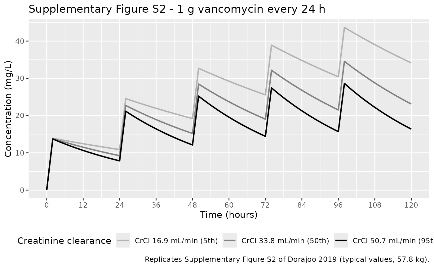
# Landmarks digitised from Supplementary Figure S2 (mg/L).
digitised <- tibble::tribble(
  ~stratum, ~time, ~published,
  "CrCl 16.9 mL/min (5th)", 2.0, 14.17,
  "CrCl 16.9 mL/min (5th)", 23.8, 10.59,
  "CrCl 16.9 mL/min (5th)", 47.8, 18.53,
  "CrCl 16.9 mL/min (5th)", 98.3, 42.62,
  "CrCl 16.9 mL/min (5th)", 119.6, 33.46,
  "CrCl 33.8 mL/min (50th)", 2.0, 14.02,
  "CrCl 33.8 mL/min (50th)", 23.8, 8.69,
  "CrCl 33.8 mL/min (50th)", 47.8, 14.17,
  "CrCl 33.8 mL/min (50th)", 98.3, 33.24,
  "CrCl 33.8 mL/min (50th)", 119.6, 22.33,
  "CrCl 50.7 mL/min (95th)", 2.0, 13.34,
  "CrCl 50.7 mL/min (95th)", 23.8, 7.14,
  "CrCl 50.7 mL/min (95th)", 47.8, 10.98,
  "CrCl 50.7 mL/min (95th)", 98.3, 27.37,
  "CrCl 50.7 mL/min (95th)", 119.6, 15.72
)

figS2 <- digitised |>
  dplyr::rowwise() |>
  dplyr::mutate(
    simulated = {
      s <- sim_typ[sim_typ$stratum == stratum, ]
      s$Cc[which.min(abs(s$time - time))]
    }
  ) |>
  dplyr::ungroup() |>
  dplyr::mutate(pct_diff = 100 * (simulated - published) / published)

# This gate is typical-value (no cohort draw), so it is not subject to the
# thread-count cohort problem. Its tolerance has to absorb two stated
# approximations rather than simulation noise: the ~2% figure digitisation
# error, and the fact that the true 5th/95th CrCl percentiles are unpublished
# and approximated as normal quantiles. Realised max |diff| is ~11% (largest
# on the 95th-percentile arm, where the normal approximation is weakest for a
# right-skewed, <60 mL/min-truncated CrCl distribution). The bound below can
# still go red: mis-transcribing Vd as the VancApp build's 0.95 L/kg moves the
# peaks by ~29%, and dropping the CrCl effect entirely moves the 5th- and
# 95th-percentile troughs by 30-40%.
stopifnot(
  abs(median(figS2$pct_diff)) < 8,
  max(abs(figS2$pct_diff)) < 20
)

figS2 |>
  dplyr::mutate(dplyr::across(c(published, simulated, pct_diff), \(x) round(x, 2))) |>
  dplyr::rename(
    "Stratum" = stratum, "Time (h)" = time,
    "Figure S2 (mg/L)" = published, "Simulated (mg/L)" = simulated,
    "% diff" = pct_diff
  ) |>
knitr::kable(caption = "Simulated vs. digitised Supplementary Figure S2 landmarks.")| Stratum | Time (h) | Figure S2 (mg/L) | Simulated (mg/L) | % diff |
|---|---|---|---|---|
| CrCl 16.9 mL/min (5th) | 2.0 | 14.17 | 13.91 | -1.84 |
| CrCl 16.9 mL/min (5th) | 23.8 | 10.59 | 10.91 | 3.00 |
| CrCl 16.9 mL/min (5th) | 47.8 | 18.53 | 19.25 | 3.88 |
| CrCl 16.9 mL/min (5th) | 98.3 | 42.62 | 43.54 | 2.15 |
| CrCl 16.9 mL/min (5th) | 119.6 | 33.46 | 34.33 | 2.60 |
| CrCl 33.8 mL/min (50th) | 2.0 | 14.02 | 13.81 | -1.49 |
| CrCl 33.8 mL/min (50th) | 23.8 | 8.69 | 9.28 | 6.78 |
| CrCl 33.8 mL/min (50th) | 47.8 | 14.17 | 15.26 | 7.71 |
| CrCl 33.8 mL/min (50th) | 98.3 | 33.24 | 34.39 | 3.46 |
| CrCl 33.8 mL/min (50th) | 119.6 | 22.33 | 23.32 | 4.43 |
| CrCl 50.7 mL/min (95th) | 2.0 | 13.34 | 13.71 | 2.81 |
| CrCl 50.7 mL/min (95th) | 23.8 | 7.14 | 7.89 | 10.57 |
| CrCl 50.7 mL/min (95th) | 47.8 | 10.98 | 12.19 | 10.99 |
| CrCl 50.7 mL/min (95th) | 98.3 | 27.37 | 28.44 | 3.93 |
| CrCl 50.7 mL/min (95th) | 119.6 | 15.72 | 16.58 | 5.49 |
Replicating Supplementary Figure S1
Supplementary Figure S1 plots the bootstrap distribution of the change in the typical value of clearance at the 5th and 95th percentiles of the cohort’s CrCl distribution, relative to the reference. The densities span roughly 0.40-0.80 (5th percentile) and 1.22-2.50 (95th percentile), with modes near 0.66 and 1.45; the shaded band marks the paper’s +/- 20% “clinically relevant” region, which both distributions clear.
ratio_at <- function(crcl) cl_at(crcl) / cl_at(33.8)

figS1 <- tibble::tibble(
  Percentile = c("5th", "95th"),
  CRCL = c(16.9, 50.7),
  `Figure S1 range` = c("0.40 - 0.80", "1.22 - 2.50"),
  `Figure S1 mode` = c(0.66, 1.45),
  Simulated = round(c(ratio_at(16.9), ratio_at(50.7)), 3)
)

# Containment check against the ranges the figure's densities actually span.
# A power or exponential CrCl form, a sign error, or a dropped covariate effect
# all land outside these intervals.
stopifnot(
  figS1$Simulated[1] > 0.40, figS1$Simulated[1] < 0.80,
  figS1$Simulated[2] > 1.22, figS1$Simulated[2] < 2.50,
  # Both extremes must clear the paper's +/- 20% relevance band, which is the
  # criterion by which CrCl was declared a significant covariate.
  figS1$Simulated[1] < 0.80, figS1$Simulated[2] > 1.20
)

knitr::kable(figS1, caption = "Clearance change at the CrCl extremes vs. Supplementary Figure S1.")| Percentile | CRCL | Figure S1 range | Figure S1 mode | Simulated |
|---|---|---|---|---|
| 5th | 16.9 | 0.40 - 0.80 | 0.66 | 0.611 |
| 95th | 50.7 | 1.22 - 2.50 | 1.45 | 1.389 |
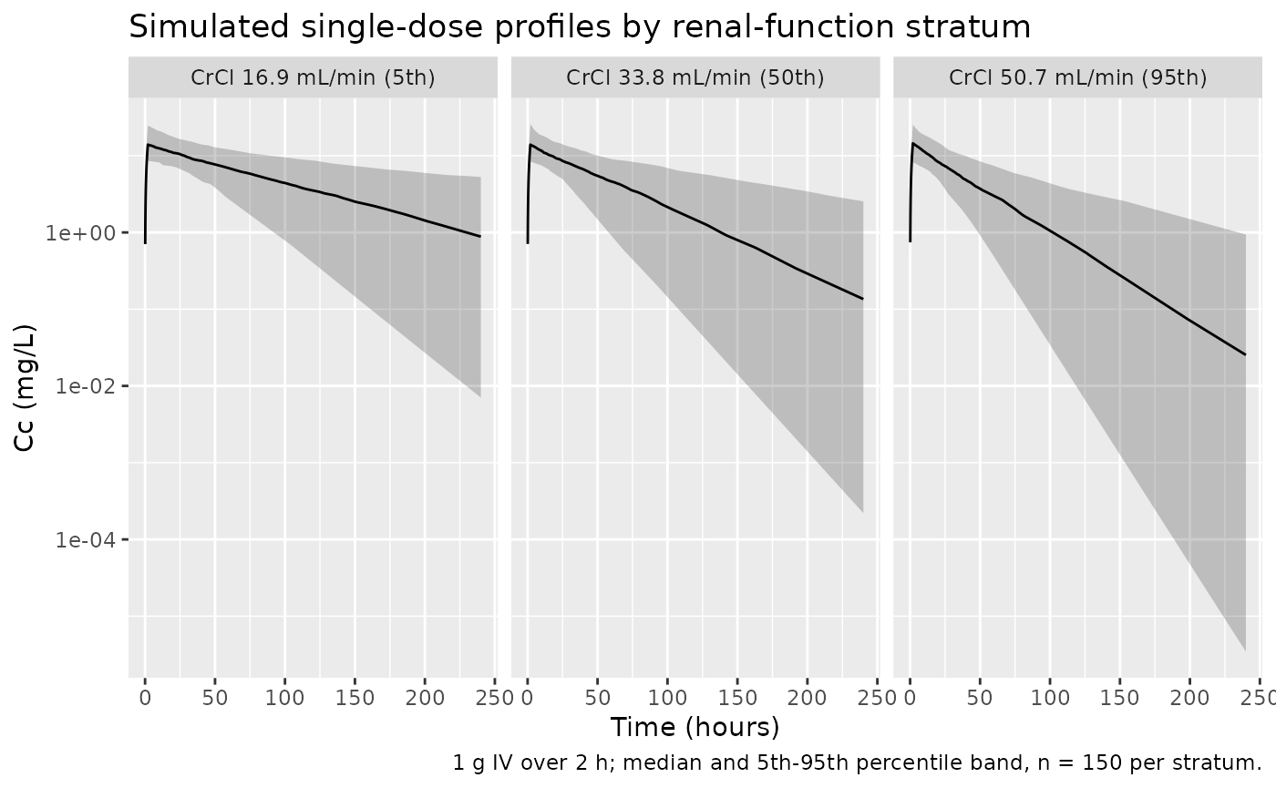
Virtual cohort
Original observed data are not publicly available. The cohort below
draws weight and Cockcroft-Gault CrCl from the construction-cohort
moments in Table 1, truncated to the study’s eligibility window (CrCl
< 60 mL/min) and to physiologically sensible weights. Each subject
receives a single 1 g infusion at the protocol maximum rate of 500 mg/h,
which supports an exact AUC(0-inf) = Dose / CL check
downstream.
# set.seed() seeds R's RNG, not rxode2's; rxode2 partitions its streams per
# solver thread, so this cohort differs between a 2-core CI runner and a
# 16-thread workstation. Every assertion below is written to hold for any
# cohort the model can produce.
set.seed(20190611)

n_per_arm <- 150L # <= 200/arm cap

make_cohort <- function(n, crcl_mean, label, id_offset = 0L) {
  tibble::tibble(
    id = id_offset + seq_len(n),
    stratum = label,
    WT = pmin(pmax(rnorm(n, 57.8, 15.7), 35), 105),
    CRCL = pmin(pmax(rnorm(n, crcl_mean, 10.3), 5), 59.9)
  )
}

subjects <- dplyr::bind_rows(
  make_cohort(n_per_arm, 16.9, "CrCl 16.9 mL/min (5th)", id_offset = 0L),
  make_cohort(n_per_arm, 33.8, "CrCl 33.8 mL/min (50th)", id_offset = 1000L),
  make_cohort(n_per_arm, 50.7, "CrCl 50.7 mL/min (95th)", id_offset = 2000L)
)

# Dense early sampling resolves the infusion peak (so trapezoidal AUC is not
# biased low); the long tail lets lambda.z extrapolate a negligible fraction.
obs_times <- sort(unique(c(
  seq(0, 12, by = 0.1), seq(12, 48, by = 0.5),
  seq(48, 240, by = 2), seq(240, 960, by = 8)
)))

events <- dplyr::bind_rows(
  subjects |> dplyr::mutate(time = 0, amt = 1000, rate = 500, evid = 1L, cmt = "central"),
  subjects |>
    tidyr::crossing(time = obs_times) |>
    dplyr::mutate(amt = NA_real_, rate = NA_real_, evid = 0L, cmt = "central")
) |>
  dplyr::arrange(id, time, dplyr::desc(evid))

stopifnot(!anyDuplicated(unique(events[, c("id", "time", "evid")])))
Simulation
sim <- rxode2::rxSolve(mod, events = events, keep = c("stratum", "WT", "CRCL")) |>
  as.data.frame()
#> ℹ parameter labels from comments will be replaced by 'label()'

stopifnot(all(sim$Cc[sim$time > 0] >= 0))
sim |>
  dplyr::filter(time > 0, time <= 240) |>
  dplyr::group_by(stratum, time) |>
  dplyr::summarise(
    Q05 = quantile(Cc, 0.05), Q50 = median(Cc), Q95 = quantile(Cc, 0.95),
    .groups = "drop"
  ) |>
  ggplot(aes(time, Q50)) +
  geom_ribbon(aes(ymin = Q05, ymax = Q95), alpha = 0.25) +
  geom_line() +
  facet_wrap(~stratum) +
  scale_y_log10() +
  labs(
    x = "Time (hours)", y = "Cc (mg/L)",
    title = "Simulated single-dose profiles by renal-function stratum",
    caption = "1 g IV over 2 h; median and 5th-95th percentile band, n = 150 per stratum."
  )
PKNCA validation
The paper reports no NCA table, so the comparison below is against the model’s own exact closed forms. For a linear one-compartment IV model these are identities, which makes the check a stringent test of the whole event-table / solve / NCA pipeline rather than a loose plausibility screen:
AUC(0-inf) = Dose / CL-
Cmax = (Rate / CL) * (1 - exp(-k * Tinf)), reached at the end of infusion t(1/2) = log(2) / k
Because eta is log-normal with median 1, the
median of each of these quantities across a stratum
equals its typical value, so the per-stratum reference is computed at
the stratum’s typical covariates.
# Filter with !is.na(Cc) ONLY -- adding time > 0 or Cc > 0 would drop the
# time-zero anchor PKNCA needs for AUC.
sim_nca <- sim |>
  dplyr::filter(!is.na(Cc)) |>
  dplyr::select(id, time, Cc, stratum)

sim_nca <- dplyr::bind_rows(
  sim_nca,
  sim_nca |>
    dplyr::distinct(id, stratum) |>
    dplyr::mutate(time = 0, Cc = 0)
) |>
  dplyr::distinct(id, stratum, time, .keep_all = TRUE) |>
  dplyr::arrange(id, stratum, time)

dose_df <- events |>
  dplyr::filter(evid == 1) |>
  dplyr::select(id, time, amt, stratum)

conc_obj <- PKNCA::PKNCAconc(sim_nca, Cc ~ time | stratum + id,
  concu = "mg/L", timeu = "h"
)
dose_obj <- PKNCA::PKNCAdose(dose_df, amt ~ time | stratum + id, doseu = "mg")

intervals <- data.frame(
  start = 0, end = Inf,
  cmax = TRUE, tmax = TRUE, aucinf.obs = TRUE, half.life = TRUE
)

nca_res <- PKNCA::pk.nca(PKNCA::PKNCAdata(conc_obj, dose_obj, intervals = intervals))
published <- strata |>
  dplyr::transmute(
    stratum,
    cl = cl_at(CRCL),
    v = v_at(WT),
    k = cl / v,
    cmax = (rate / cl) * (1 - exp(-k * tinf)),
    tmax = tinf,
    aucinf.obs = 1000 / cl,
    half.life = log(2) / k
  ) |>
  dplyr::select(stratum, cmax, tmax, aucinf.obs, half.life)

cmp <- nlmixr2lib::ncaComparisonTable(
  simulated = nca_res,
  reference = published,
  by = "stratum",
  units = c(
    cmax = "mg/L", aucinf.obs = "mg*h/L",
    tmax = "h", half.life = "h"
  ),
  tolerance_pct = 20
)

knitr::kable(
  cmp,
  caption = "Simulated (PKNCA, median across subjects) vs. closed-form typical values. * differs by >20%.",
  align = c("l", "l", "r", "r", "r")
)| NCA parameter | stratum | Reference | Simulated | % diff |
|---|---|---|---|---|
| Cmax (mg/L) | CrCl 16.9 mL/min (5th) | 13.9 | 14 | +0.3% |
| Cmax (mg/L) | CrCl 33.8 mL/min (50th) | 13.8 | 13.9 | +0.8% |
| Cmax (mg/L) | CrCl 50.7 mL/min (95th) | 13.7 | 14.5 | +5.8% |
| Tmax (h) | CrCl 16.9 mL/min (5th) | 2 | 2 | +0.0% |
| Tmax (h) | CrCl 33.8 mL/min (50th) | 2 | 2 | +0.0% |
| Tmax (h) | CrCl 50.7 mL/min (95th) | 2 | 2 | +0.0% |
| AUC0-∞ (obs) (mg*h/L) | CrCl 16.9 mL/min (5th) | 1260 | 1270 | +1.2% |
| AUC0-∞ (obs) (mg*h/L) | CrCl 33.8 mL/min (50th) | 769 | 808 | +5.1% |
| AUC0-∞ (obs) (mg*h/L) | CrCl 50.7 mL/min (95th) | 554 | 546 | -1.4% |
| t½ (h) | CrCl 16.9 mL/min (5th) | 62 | 59.3 | -4.4% |
| t½ (h) | CrCl 33.8 mL/min (50th) | 37.9 | 36.4 | -4.1% |
| t½ (h) | CrCl 50.7 mL/min (95th) | 27.3 | 26 | -4.8% |
# Per-subject exactness: for an IV model AUC(0-inf) * CL == Dose identically,
# subject by subject. This is a within-subject identity (same drawn CL on both
# sides), so the only error is trapezoidal + lambda.z extrapolation -- a tight
# bound is correct and it is not cohort-dependent.
auc_sub <- as.data.frame(nca_res$result) |>
  dplyr::filter(PPTESTCD == "aucinf.obs") |>
  dplyr::select(id, stratum, auc = PPORRES) |>
  dplyr::left_join(
    sim |> dplyr::distinct(id, cl),
    by = "id"
  ) |>
  dplyr::mutate(recovery = auc * cl / 1000)

stopifnot(nrow(auc_sub) == nrow(subjects), !anyNA(auc_sub$recovery))
stopifnot(
  abs(median(auc_sub$recovery) - 1) < 0.01,
  max(abs(auc_sub$recovery - 1)) < 0.05
)

# The stratum medians must track the closed-form typical values. Sampling error
# on a median of n = 150 with 54% CV on CL is roughly 5-6%, so 15% leaves
# headroom for any cohort while still failing on a mis-scaled clearance.
cmp_num <- cmp |>
  dplyr::filter(!is.na(`% diff`)) |>
  dplyr::mutate(pd = as.numeric(gsub("[^0-9.+-]", "", as.character(`% diff`))))
stopifnot(max(abs(cmp_num$pd), na.rm = TRUE) < 15)

c(
  median_auc_recovery = median(auc_sub$recovery),
  worst_subject_recovery = auc_sub$recovery[which.max(abs(auc_sub$recovery - 1))]
)
#>    median_auc_recovery worst_subject_recovery
#>              0.9999997              0.9999808
Assumptions and deviations
-
Functional form of the CrCl effect on clearance.
Table 2 reports
theta CrCl = 0.023but the paper never prints the covariate equation, and the Supplementary Methods say continuous covariates were screened as “linear, power and exponential functions” without stating which won. Three independent lines of evidence fix the form as the centred linear one used here,CL = 1.30 * (1 + 0.023 * (CrCl - ref)):- The authors’ own deposited VancApp
server.R(Supplementary R code) codes exactly this shape:CL <- 1.4*( 1 + 0.0224*(CRCL - 35.75)). - Digitising Supplementary Figure S2 and solving each curve jointly for CL and V gives CL = 0.79 / 1.31 / 1.90 L/h and V = 69.8 / 70.0 / 73.0 L at the 5th / 50th / 95th CrCl percentiles. The 50th-percentile CL of 1.31 L/h recovers Table 2’s 1.30 L/h, and V/57.8 = 1.21-1.26 L/kg recovers Table 2’s 1.23 L/kg. Back-solving the CrCl values these imply under the linear form gives 16.8 / 34.1 mL/min for the 5th / 50th percentiles – essentially the normal quantiles of the published CrCl distribution (16.9 / 33.8). Under an exponential form the same curves would require a 5th percentile near 12 mL/min (z = -2.1), i.e. a pronounced left skew that a CrCl distribution truncated at 60 mL/min does not have.
- Supplementary Figure S1’s CL-ratio densities (modes ~0.66 and ~1.45) match the linear form’s 0.61 and 1.39 at the normal CrCl quantiles.
- The authors’ own deposited VancApp
-
Centering constant. The paper does not print the
CrCl value at which
Cl = 1.30 L/happlies. It is set here to 33.8 mL/min, the construction-cohort mean CrCl from Table 1 – the only CrCl reference the paper publishes for the estimation cohort, and the value the Figure S2 digitisation supports (the 50th-percentile curve’s clearance recovers 1.30 L/h at 34.1 mL/min). The VancApp code centres at 35.75 mL/min instead; see the next bullet for why that build’s constants were not adopted. -
The deposited VancApp code is a preliminary build, not the
final model. Its
server.RcarriesPOPCL <- 1.4,POPV1 <- 0.95,theta = 0.0224,ref = 35.75, and IIV standard deviations of 0.202 (CL) and 0.0855 (V) – none of which match Table 2’s 1.30 L/h, 1.23 L/kg, 0.023, 54.4% and 22.5%. Per the standing rule that a paper’s published results table supersedes a deposited control stream or application build, every numeric value packaged here comes from Table 2; the code is used only as evidence of the equation form. Users reproducing VancApp’s exact output will see roughly 8% higher clearance and 23% lower volume than this model gives. -
IIV scale. Table 2 reports the random effects as
percentages (“eta Cl (%) 54.4”, “eta Vd (%) 22.5”) without stating
whether these are omega or CV. They are read as coefficients of
variation and converted with
omega^2 = log(CV^2 + 1), the convention for exponential (log-normal) IIV stated in the Methods. The alternative reading (percentages as omega directly) would give omega^2 of 0.2959 and 0.0506 rather than 0.2593 and 0.0494 – a difference of 14% and 3% in the variances, too small for any published figure to discriminate. -
Residual error scale. Table 2 labels the additive
term “(mg/L)” and the proportional term “(sigma^2)”. The additive term
is therefore taken as a standard deviation in mg/L (2.46) and the
proportional term as a variance, so
propSd = sqrt(0.001) = 0.0316. The Methods describe a “mixture of additive and proportional error structures”, encoded as nlmixr2’s combined error. -
CrCl units. Table 1 labels the row “Creatinine
clearance* (ml/min/1.73 m2)”, but Cockcroft-Gault is not a
BSA-normalised estimator; Table 3 labels the same quantity “(ml/min)”
and the VancApp code computes raw Cockcroft-Gault with no BSA term. The
CRCLcolumn is therefore documented and used as raw mL/min, and the “/1.73 m2” in Table 1 is treated as a labelling error. -
Unpublished CrCl percentiles. Supplementary Figure
S2’s 5th/50th/95th percentile values are not printed. They are
approximated here as
33.8 -/+ 1.645 * 10.3= 16.9 / 33.8 / 50.7 mL/min. This is the dominant source of the residual disagreement in the Figure S2 gate (up to 11% on the 95th-percentile arm, where a right-skewed distribution truncated at 60 mL/min departs most from the normal approximation). -
Digitised reference values. The Supplementary
Figure S1 and S2 reference numbers in this vignette were obtained by
programmatic digitisation of the supplement’s figure images
(gridline-calibrated axis mapping, grey-level curve tracing); read
accuracy is about +/- 2%. They are not printed anywhere in the paper. No
packaged
ini()value depends on them – they are used only as validation targets and as corroboration of the covariate form. -
Screened but unretained covariates. Age, sex,
height, BMI, BSA, serum creatinine, Jelliffe CrCl, MDRD and CKD-EPI
eGFR, serum albumin, C-reactive protein, procalcitonin, white cell count
and neutrophil percentage were all screened (Supplementary Methods) and
none reached significance: “All other potential covariates tested were
insignificant.” They are recorded in the model file’s
covariatesDataExcludedmetadata with no point estimates, since none are published. Neutrophil percentage has no canonical covariate column ininst/references/covariate-columns.mdand is documented in prose within theWBCentry rather than given one. -
Sex enters only through CrCl. Sex is not a
covariate on any PK parameter, but the Cockcroft-Gault CrCl that drives
clearance carries the usual 0.85 female multiplier. Users supplying
CRCLmust apply it upstream. - Applicability domain. Eligibility required CrCl < 60 mL/min and excluded renal replacement therapy, so extrapolating this model above 60 mL/min or to dialysis patients is unsupported; VancApp itself emits a warning above 60 mL/min. The linear CL multiplier remains positive down to CrCl = 0 (0.223 at zero), so the model is numerically safe across the physiological range even though it is only validated below 60.
- Cohort simulation choices. Weight and CrCl are drawn independently from the Table 1 marginal moments; the paper publishes no correlation between them, although Cockcroft-Gault CrCl is mechanistically weight-dependent, so the virtual cohort’s joint distribution is wider than the real one. Weight is truncated to 35-105 kg (near the published 33.6-103.8 range) and CrCl to 5-59.9 mL/min (the eligibility ceiling).
- What is not packaged. The paper’s Phase 3 clinical-impact analysis (time-to-target trough, 30-day mortality, nephrotoxicity) is an outcomes comparison with no model, and the VancApp dose-adjustment module is a Bayesian forecasting interface over the same PK model. Neither adds a distinct structural model, so only the Table 2 population PK model is packaged.