PEGylated asparaginase and anti-PEG IgM (Siebel 2022)
Source:vignettes/articles/Siebel_2022_pegasparaginase.Rmd
Siebel_2022_pegasparaginase.RmdModel and source
Siebel 2022 asks whether antibodies against polyethylene glycol (PEG)
change the pharmacokinetics of PEGylated asparaginase (PEG-ASNase) in
children with acute lymphoblastic leukaemia treated in the AIEOP-BFM ALL
2009 trial. The authors took their group’s previously published
population PK model (the 14-compartment de-PEGylation transit chain of
Wurthwein 2021) as a reference model, refitted it to the
antibody data set, and screened anti-PEG IgG and IgM measured before and
after dosing as covariates on the initial clearance
CLinitial. The final model adds a single effect: a
hockey stick on the natural-log pre-existing anti-PEG IgM
level, active only above an estimated cut point and only at the
first induction dose.
- Citation: Siebel C, Lanvers-Kaminsky C, Alten J, Smisek P, Nath CE, Rizzari C, Boos J, Wurthwein G. Impact of Antibodies Against Polyethylene Glycol on the Pharmacokinetics of PEGylated Asparaginase in Children with Acute Lymphoblastic Leukaemia: A Population Pharmacokinetic Approach. Eur J Drug Metab Pharmacokinet. 2022;47(2):187-198. doi:10.1007/s13318-021-00741-w
- Article: https://doi.org/10.1007/s13318-021-00741-w
- Supplement (NONMEM control stream of the final model in Section 3): Electronic Supplementary Material 1 at the same DOI.
The package also ships the later models of the same group,
Wurthwein_2025_pegasparaginase_*, fitted to a larger
AIEOP-BFM ALL 2009 data set. Two of them carry the same IgM hockey stick
with the cut point estimated here (1.30 on the log scale) held
fixed.
mod <- rxode2::rxode(readModelDb("Siebel_2022_pegasparaginase"))
#> ℹ parameter labels from comments will be replaced by 'label()'
#> Warning: some etas defaulted to non-mu referenced, possible parsing error: etaiov_vc_1, etaiov_vc_2, etaiov_vc_3, etaiov_cl_1, etaiov_cl_2, etaiov_cl_3
#> as a work-around try putting the mu-referenced expression on a simple line
mod0 <- rxode2::zeroRe(mod)
#> Warning: some etas defaulted to non-mu referenced, possible parsing error: etaiov_vc_1, etaiov_vc_2, etaiov_vc_3, etaiov_cl_1, etaiov_cl_2, etaiov_cl_3
#> as a work-around try putting the mu-referenced expression on a simple line
Population
1444 children with acute lymphoblastic leukaemia from the German and Czech part of AIEOP-BFM ALL 2009 (EudraCT 2007-004270-43), who received 3403 PEG-ASNase administrations: two induction doses on protocol IA days 12 and 26 (all patients) and one re-induction dose on protocol II day 8 (non-high-risk patients only), each 2500 U/m^2 as a 2-hour infusion with a 3750 U cap. Median age 5.13 years (range 1.06-18.32), median body surface area (BSA) 0.78 m^2 (0.41-2.58), 842 male / 602 female (Table 1). 6261 activity samples were analysed, drawn mostly 7 and 14 days after each dose (ESM Table S1), together with 2082 pre-dose and 6412 post-dose anti-PEG antibody measurements (Table 2). Median pre-existing anti-PEG IgM before induction was 1.37 mean fluorescence intensity (MFI), range 0.19-18.1; 146 of the 1444 patients were above the finally estimated cut point of 3.67 MFI.
Samples at or after a hypersensitivity reaction or silent inactivation were excluded before fitting, so the model describes standard elimination only.
The same information is available programmatically via
readModelDb("Siebel_2022_pegasparaginase")()$population.
Structural model
Asparaginase activity is carried by a chain of 14 serial compartments
that share one serum volume V. Drug steps from compartment
i to i+1 at Qtr/V (standing in for
progressive hydrolysis of the PEG moiety) and every compartment is
eliminated at CLinitial/V; the terminal compartment passes
its Qtr/V out of the system. Apparent clearance therefore
rises within a dosing interval from CLinitial towards
CLinitial + Qtr as mass migrates down the chain. The assay
measures total catalytic activity, so the observation is
Cc = (central + transit1 + ... + transit13) / V. All of
this is read directly off the $DES and $ERROR
blocks in ESM Section 3.
Covariates act on V, CLinitial and
Qtr exactly as in the control stream:
- BSA enters linearly, centred on 0.79 m^2
(
THETA(1) * (1 + SCV1 * (BSA - 0.79))), with one slope forVand one shared byCLinitialandQtr. - Age above 8 years increases
CLinitiallinearly; females have 7% lowerCLinitial. -
VandCLinitialchange stepwise at the second induction dose and at re-induction, relative to the first induction dose. - Anti-PEG IgM:
CLinitialis multiplied by1 + 0.414 * max(log(IgM) - 1.30, 0)at the first induction dose only.
The anti-PEG IgM hockey stick
Section 3.3 states the effect in one sentence: “each additional log
unit of anti-PEG IgMprior above the estimated cut point (i.e. an
increase in anti-PEG IgMprior from 1.30 to 2.30 on the log scale or,
equivalently, from 3.67 to 9.97 on the linear scale) was related to an
increase in CLinitial of 41.4%”. The chunk below reads the individual
cl back out of solved model output across a range of IgM
levels, so it checks the encoding as it runs, not a re-derivation of
it.
igm_grid <- c(0.19, 0.5, 1, 1.37, 2, 3, 3.67, 5, 7, 9.97, 12, 15, 18.1)

cl_at <- function(igm, occ) {
  ev <- rxode2::et(amt = 1950, dur = 2 / 24, cmt = "central") |>
    rxode2::et(1, cmt = "central") |>
    as.data.frame() |>
    mutate(BSA = 0.78, AGE = 5.13, SEXF = 0, OCC = occ, ABPEG_IGM = igm)
  s <- rxode2::rxSolve(mod0, ev, returnType = "data.frame")
  s$cl[s$time == 1]
}

cl_ref <- cl_at(1, 1)
#> ℹ omega/sigma items treated as zero: 'etalcl', 'etaiov_vc_1', 'etaiov_vc_2', 'etaiov_vc_3', 'etaiov_cl_1', 'etaiov_cl_2', 'etaiov_cl_3'
igm_tab <- tidyr::expand_grid(igm = igm_grid, occ = c(1, 2)) |>
  rowwise() |>
  mutate(cl_rel = cl_at(igm, occ) / (cl_ref * ifelse(occ == 2, 1 - 0.107, 1))) |>
  ungroup()
#> ℹ omega/sigma items treated as zero: 'etalcl', 'etaiov_vc_1', 'etaiov_vc_2', 'etaiov_vc_3', 'etaiov_cl_1', 'etaiov_cl_2', 'etaiov_cl_3'
#> ℹ omega/sigma items treated as zero: 'etalcl', 'etaiov_vc_1', 'etaiov_vc_2', 'etaiov_vc_3', 'etaiov_cl_1', 'etaiov_cl_2', 'etaiov_cl_3'
#> ℹ omega/sigma items treated as zero: 'etalcl', 'etaiov_vc_1', 'etaiov_vc_2', 'etaiov_vc_3', 'etaiov_cl_1', 'etaiov_cl_2', 'etaiov_cl_3'
#> ℹ omega/sigma items treated as zero: 'etalcl', 'etaiov_vc_1', 'etaiov_vc_2', 'etaiov_vc_3', 'etaiov_cl_1', 'etaiov_cl_2', 'etaiov_cl_3'
#> ℹ omega/sigma items treated as zero: 'etalcl', 'etaiov_vc_1', 'etaiov_vc_2', 'etaiov_vc_3', 'etaiov_cl_1', 'etaiov_cl_2', 'etaiov_cl_3'
#> ℹ omega/sigma items treated as zero: 'etalcl', 'etaiov_vc_1', 'etaiov_vc_2', 'etaiov_vc_3', 'etaiov_cl_1', 'etaiov_cl_2', 'etaiov_cl_3'
#> ℹ omega/sigma items treated as zero: 'etalcl', 'etaiov_vc_1', 'etaiov_vc_2', 'etaiov_vc_3', 'etaiov_cl_1', 'etaiov_cl_2', 'etaiov_cl_3'
#> ℹ omega/sigma items treated as zero: 'etalcl', 'etaiov_vc_1', 'etaiov_vc_2', 'etaiov_vc_3', 'etaiov_cl_1', 'etaiov_cl_2', 'etaiov_cl_3'
#> ℹ omega/sigma items treated as zero: 'etalcl', 'etaiov_vc_1', 'etaiov_vc_2', 'etaiov_vc_3', 'etaiov_cl_1', 'etaiov_cl_2', 'etaiov_cl_3'
#> ℹ omega/sigma items treated as zero: 'etalcl', 'etaiov_vc_1', 'etaiov_vc_2', 'etaiov_vc_3', 'etaiov_cl_1', 'etaiov_cl_2', 'etaiov_cl_3'
#> ℹ omega/sigma items treated as zero: 'etalcl', 'etaiov_vc_1', 'etaiov_vc_2', 'etaiov_vc_3', 'etaiov_cl_1', 'etaiov_cl_2', 'etaiov_cl_3'
#> ℹ omega/sigma items treated as zero: 'etalcl', 'etaiov_vc_1', 'etaiov_vc_2', 'etaiov_vc_3', 'etaiov_cl_1', 'etaiov_cl_2', 'etaiov_cl_3'
#> ℹ omega/sigma items treated as zero: 'etalcl', 'etaiov_vc_1', 'etaiov_vc_2', 'etaiov_vc_3', 'etaiov_cl_1', 'etaiov_cl_2', 'etaiov_cl_3'
#> ℹ omega/sigma items treated as zero: 'etalcl', 'etaiov_vc_1', 'etaiov_vc_2', 'etaiov_vc_3', 'etaiov_cl_1', 'etaiov_cl_2', 'etaiov_cl_3'
#> ℹ omega/sigma items treated as zero: 'etalcl', 'etaiov_vc_1', 'etaiov_vc_2', 'etaiov_vc_3', 'etaiov_cl_1', 'etaiov_cl_2', 'etaiov_cl_3'
#> ℹ omega/sigma items treated as zero: 'etalcl', 'etaiov_vc_1', 'etaiov_vc_2', 'etaiov_vc_3', 'etaiov_cl_1', 'etaiov_cl_2', 'etaiov_cl_3'
#> ℹ omega/sigma items treated as zero: 'etalcl', 'etaiov_vc_1', 'etaiov_vc_2', 'etaiov_vc_3', 'etaiov_cl_1', 'etaiov_cl_2', 'etaiov_cl_3'
#> ℹ omega/sigma items treated as zero: 'etalcl', 'etaiov_vc_1', 'etaiov_vc_2', 'etaiov_vc_3', 'etaiov_cl_1', 'etaiov_cl_2', 'etaiov_cl_3'
#> ℹ omega/sigma items treated as zero: 'etalcl', 'etaiov_vc_1', 'etaiov_vc_2', 'etaiov_vc_3', 'etaiov_cl_1', 'etaiov_cl_2', 'etaiov_cl_3'
#> ℹ omega/sigma items treated as zero: 'etalcl', 'etaiov_vc_1', 'etaiov_vc_2', 'etaiov_vc_3', 'etaiov_cl_1', 'etaiov_cl_2', 'etaiov_cl_3'
#> ℹ omega/sigma items treated as zero: 'etalcl', 'etaiov_vc_1', 'etaiov_vc_2', 'etaiov_vc_3', 'etaiov_cl_1', 'etaiov_cl_2', 'etaiov_cl_3'
#> ℹ omega/sigma items treated as zero: 'etalcl', 'etaiov_vc_1', 'etaiov_vc_2', 'etaiov_vc_3', 'etaiov_cl_1', 'etaiov_cl_2', 'etaiov_cl_3'
#> ℹ omega/sigma items treated as zero: 'etalcl', 'etaiov_vc_1', 'etaiov_vc_2', 'etaiov_vc_3', 'etaiov_cl_1', 'etaiov_cl_2', 'etaiov_cl_3'
#> ℹ omega/sigma items treated as zero: 'etalcl', 'etaiov_vc_1', 'etaiov_vc_2', 'etaiov_vc_3', 'etaiov_cl_1', 'etaiov_cl_2', 'etaiov_cl_3'
#> ℹ omega/sigma items treated as zero: 'etalcl', 'etaiov_vc_1', 'etaiov_vc_2', 'etaiov_vc_3', 'etaiov_cl_1', 'etaiov_cl_2', 'etaiov_cl_3'
#> ℹ omega/sigma items treated as zero: 'etalcl', 'etaiov_vc_1', 'etaiov_vc_2', 'etaiov_vc_3', 'etaiov_cl_1', 'etaiov_cl_2', 'etaiov_cl_3'

ggplot(igm_tab, aes(igm, cl_rel, linetype = factor(occ))) +
  geom_line() +
  geom_point(data = filter(igm_tab, occ == 1)) +
  geom_vline(xintercept = 3.67, linetype = "dotted") +
  scale_x_log10() +
  scale_linetype_manual(values = c("1" = "solid", "2" = "dashed"),
                        labels = c("1" = "1st induction dose", "2" = "2nd induction dose")) +
  labs(x = "Pre-existing anti-PEG IgM (MFI, log axis)",
       y = "CLinitial relative to below-cut-point patient", linetype = NULL) +
  theme_bw()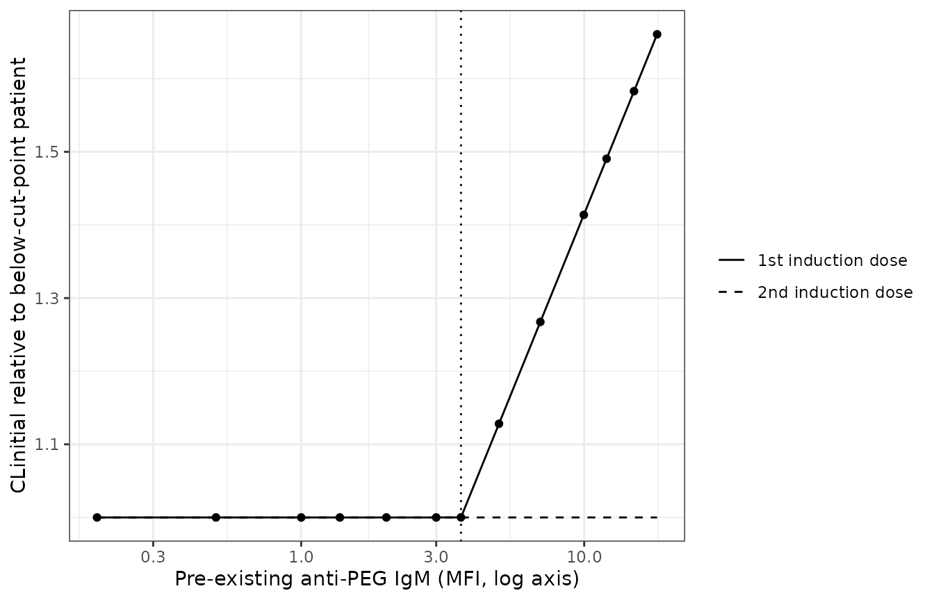
Initial clearance relative to a patient below the cut point, as a function of the pre-existing anti-PEG IgM level, at the first induction dose (solid) and at the second induction dose (dashed). Model-derived from Siebel 2022 Table 3 and ESM Section 3.
f <- function(igm, occ = 1) igm_tab$cl_rel[igm_tab$igm == igm & igm_tab$occ == occ]
c(at_median_1.37 = f(1.37), at_cut_3.67 = f(3.67), one_log_above_9.97 = f(9.97),
  max_18.1 = f(18.1), second_dose_at_18.1 = f(18.1, 2))
#>      at_median_1.37         at_cut_3.67  one_log_above_9.97            max_18.1
#>            1.000000            1.000079            1.413826            1.660708
#> second_dose_at_18.1
#>            1.000000

stopifnot(
  # Below the cut point there is no effect. 3.67 is the paper's rounding of
  # exp(1.30) = 3.6693, so it sits 0.0002 log units above the cut point and
  # its factor is 1.00008; hence the bound.
  all(abs(igm_tab$cl_rel[igm_tab$igm < 3.67] - 1) < 1e-9),
  abs(f(3.67) - 1) < 5e-4,
  # 9.97 MFI is one natural-log unit above 3.67, so the factor is 1 + 0.414
  # exactly (Section 3.3, '41.4%'); the tolerance only absorbs the rounding of
  # 3.67 and 9.97 in the text.
  abs(f(9.97) - 1.414) < 0.002,
  # The effect is restricted to the first induction dose.
  all(abs(igm_tab$cl_rel[igm_tab$occ == 2] - 1) < 1e-6)
)
Mass balance
A linear chain has a closed-form total AUC. With
ke = CLinitial/V, kt = Qtr/V and
ratio = kt/(ke + kt), a dose D gives
AUC = D / (V * (ke + kt)) * sum(ratio^j, j = 0..13).
Reproducing it from the solved ODEs confirms that the chain is wired
correctly and conserves mass.
ev_mb <- rxode2::et(amt = 1950, cmt = "central") |>
  rxode2::et(seq(0, 150, by = 0.01), cmt = "central") |>
  as.data.frame() |>
  mutate(BSA = 0.78, AGE = 5.13, SEXF = 0, OCC = 1, ABPEG_IGM = 9.97)
mb <- rxode2::rxSolve(mod0, ev_mb, returnType = "data.frame")
#> ℹ omega/sigma items treated as zero: 'etalcl', 'etaiov_vc_1', 'etaiov_vc_2', 'etaiov_vc_3', 'etaiov_cl_1', 'etaiov_cl_2', 'etaiov_cl_3'

auc_num <- sum(diff(mb$time) * (head(mb$Cc, -1) + tail(mb$Cc, -1)) / 2)
V <- mb$vc[1]; ke <- mb$cl[1] / V; kt <- mb$q[1] / V; r <- kt / (ke + kt)
auc_cf <- 1950 / (V * (ke + kt)) * sum(r^(0:13))

c(numeric = auc_num, closed_form = auc_cf, pct_diff = 100 * (auc_num - auc_cf) / auc_cf)
#>      numeric  closed_form     pct_diff
#> 1.309879e+04 1.309879e+04 1.061958e-05

# A solve against its own closed form is pure numerical error, so the bound is
# tight: no per-subject random mechanism enters either side.
stopifnot(abs(auc_num - auc_cf) / auc_cf < 0.005)
Source trace
Every ini() entry carries an in-file comment naming its
source location.
| Item | Value(s) | Source location |
|---|---|---|
Chain of 14 serial compartments; dose into compartment 1; shared
V
|
topology | ESM Section 3 $MODEL, $DES; ESM Fig.
S1 |
Observation = total activity over all 14 states divided by
V
|
structural | ESM Section 3 $ERROR
(TOT = A(1)+...+A(14); IPRED = TOT/V1) |
V, CLinitial, Qtr
|
1.71 L, 0.128 L/day, 0.954 L/day (at BSA 1 m^2) | Table 3, final covariate model |
BSA linear, centred on 0.79 m^2; slopes on V and on
CLinitial + Qtr
|
1.60, 1.49 | ESM Section 3 $PK; Table 3 and footnote (a) |
| Quoting convention: values reported for BSA = 1 m^2 | convention | Table 3, note under the table |
Phase changes in V (2nd induction dose,
re-induction) |
-0.158, -0.288 | Table 3 and footnote (b); ESM Section 3 V1KOV
|
Phase changes in CLinitial (2nd induction dose,
re-induction) |
-0.107, -0.438 | Table 3 and footnote (b); ESM Section 3 CLKOV
|
| Age hockey stick, break point fixed at 8 years | 0.011 per year | Table 3 footnote (c); ESM Section 3 (THETA(13)
0 FIX) |
Sex on CLinitial, males the reference (SEX
1/2) |
-0.070 | Table 3 footnote (d); ESM Section 3 CLSEX
|
| Anti-PEG IgM slope above the cut point, first induction dose only | 0.414 per log unit | Table 3 footnote (e); ESM Section 3 (THETA(17),
THETA(18) 0 FIX) |
| Anti-PEG IgM cut point, natural-log scale | 1.30 (3.67 MFI) | Table 3 footnote (f); Section 3.2.1 |
IIV on CLinitial; no IIV on V or
Qtr
|
25.4% | Table 3; ESM Section 3 $OMEGA (0 FIX) |
IOV on V and CLinitial, one occasion per
administration |
11.9%, 22.8% | Table 3; ESM Section 3 $OMEGA BLOCK(1) SAME
|
| Combined proportional + additive residual error | 0.191, 5.36 U/L | Table 3; ESM Section 3 $ERROR,
$SIGMA 1 FIX
|
| Published simulated day-14 troughs used as gates below | 517, 339, 305, 194 U/L | Section 3.3; ESM Table S5; Fig. 4 |
Reproducing the published simulations
Section 3.3, ESM Table S5 and Figure 4 report Monte Carlo simulations of 1000 patients per arm, with BSA and age fixed at their medians (0.78 m^2, 5.13 years) and sex at the most frequent value (male), for two induction doses 14 days apart. Two regimens (2500 U/m^2 over 2 h; 1500 U/m^2 over 1 h) are crossed with two IgM levels: at the cut point (3.67 MFI, no effect) and one log unit above it (9.97 MFI). The published summary is the median (IQR) trough 14 days after the first dose.
published <- tibble::tribble(
  ~regimen,          ~igm,  ~median, ~q25, ~q75, ~pct_below_100,
  "2500 U/m^2, 2 h", 3.67,  517,     391,  632,  0.5,
  "2500 U/m^2, 2 h", 9.97,  339,     222,  457,  4.9,
  "1500 U/m^2, 1 h", 3.67,  305,     241,  367,  1.7,
  "1500 U/m^2, 1 h", 9.97,  194,     135,  262,  14.9
) |>
  mutate(dose_m2 = ifelse(grepl("^2500", regimen), 2500, 1500),
         dur_h   = ifelse(grepl("2 h$", regimen), 2, 1))
Typical-value troughs
bsa_med <- 0.78
trough_typical <- function(dose_m2, dur_h, igm) {
  ev <- rxode2::et(amt = dose_m2 * bsa_med, dur = dur_h / 24, cmt = "central") |>
    rxode2::et(c(7, 14), cmt = "central") |>
    as.data.frame() |>
    mutate(BSA = bsa_med, AGE = 5.13, SEXF = 0, OCC = 1, ABPEG_IGM = igm)
  s <- rxode2::rxSolve(mod0, ev, returnType = "data.frame")
  s$Cc[s$time == 14]
}

typ <- published |>
  rowwise() |>
  mutate(typical = trough_typical(dose_m2, dur_h, igm)) |>
  ungroup() |>
  mutate(pct_diff = 100 * (typical - median) / median)
#> ℹ omega/sigma items treated as zero: 'etalcl', 'etaiov_vc_1', 'etaiov_vc_2', 'etaiov_vc_3', 'etaiov_cl_1', 'etaiov_cl_2', 'etaiov_cl_3'
#> ℹ omega/sigma items treated as zero: 'etalcl', 'etaiov_vc_1', 'etaiov_vc_2', 'etaiov_vc_3', 'etaiov_cl_1', 'etaiov_cl_2', 'etaiov_cl_3'
#> ℹ omega/sigma items treated as zero: 'etalcl', 'etaiov_vc_1', 'etaiov_vc_2', 'etaiov_vc_3', 'etaiov_cl_1', 'etaiov_cl_2', 'etaiov_cl_3'
#> ℹ omega/sigma items treated as zero: 'etalcl', 'etaiov_vc_1', 'etaiov_vc_2', 'etaiov_vc_3', 'etaiov_cl_1', 'etaiov_cl_2', 'etaiov_cl_3'

typ |>
  select(regimen, igm, median, typical, pct_diff) |>
  dplyr::rename(
    "Regimen" = regimen,
    "Anti-PEG IgM (MFI)" = igm,
    "Published median (U/L)" = median,
    "Typical-value solve (U/L)" = typical,
    "Difference (%)" = pct_diff
  ) |>
  knitr::kable(digits = c(0, 2, 0, 0, 1),
caption = "Day-14 trough after the first induction dose. Published values from Section 3.3 and ESM Table S5.")| Regimen | Anti-PEG IgM (MFI) | Published median (U/L) | Typical-value solve (U/L) | Difference (%) |
|---|---|---|---|---|
| 2500 U/m^2, 2 h | 3.67 | 517 | 517 | 0.0 |
| 2500 U/m^2, 2 h | 9.97 | 339 | 333 | -1.9 |
| 1500 U/m^2, 1 h | 3.67 | 305 | 309 | 1.5 |
| 1500 U/m^2, 1 h | 9.97 | 194 | 199 | 2.6 |
stopifnot(
  # A mis-transcribed V, CLinitial, Qtr, BSA slope or antibody term moves these
  # troughs by tens of percent. The remaining gap compares a typical-value solve
  # with a 1000-patient Monte Carlo median and is under 3%. The solve is
  # deterministic, so the bound does not depend on the random-number stream.
  abs(median(typ$pct_diff)) < 3,
  max(abs(typ$pct_diff)) < 5
)
The typical-value solve lands within 3% of every published median, which is about the Monte Carlo noise of a 1000-patient median.
Which reading of the BSA quoting convention?
Table 3 reports V, CLinitial and
Qtr “for a child with BSA = 1 m^2 for better comparison”.
Because BSA enters linearly and centred on 0.79 m^2, that means the
NONMEM THETA is the printed value divided by
1 + slope * 0.21, and that is how the model file is
encoded. The predecessor paper (Wurthwein 2021) describes the same
convention differently – values “converted from L/0.79m2 to L/m2” –
which read literally gives THETA = printed * 0.79. The two
readings differ by 3-5% in the typical parameters. Siebel 2022’s own
simulations can arbitrate, because they are typical-covariate
simulations of exactly these parameters. The chain has a Poisson closed
form, so both readings can be evaluated without re-encoding the
model:
trough_cf <- function(V, CL, Q, D, t = 14) {
  ke <- CL / V; kt <- Q / V
  D * exp(-(ke + kt) * t) * sum((kt * t)^(0:13) / factorial(0:13)) / V
}
readings <- list(
  "BSA = 1 m^2 (model file)" = c(V = 1.71 / (1 + 1.60 * 0.21),
                                 CL = 0.128 / (1 + 1.49 * 0.21),
                                 Q = 0.954 / (1 + 1.49 * 0.21)),
  "printed x 0.79"           = c(V = 1.71 * 0.79, CL = 0.128 * 0.79, Q = 0.954 * 0.79)
)
bsa_cmp <- lapply(names(readings), function(nm) {
  th <- readings[[nm]]
  V  <- th[["V"]]  * (1 + 1.60 * (bsa_med - 0.79))
  CL <- th[["CL"]] * (1 + 1.49 * (bsa_med - 0.79))
  Q  <- th[["Q"]]  * (1 + 1.49 * (bsa_med - 0.79))
  published |>
    rowwise() |>
    mutate(reading = nm,
           closed_form = trough_cf(V, CL * ifelse(igm > 3.67, 1 + 0.414 * (log(igm) - 1.30), 1),
                                   Q, dose_m2 * bsa_med)) |>
    ungroup()
}) |>
  bind_rows() |>
  mutate(pct_diff = 100 * (closed_form - median) / median)

bsa_cmp |>
  group_by(reading) |>
  summarise(mean_abs_pct_diff = mean(abs(pct_diff)), .groups = "drop") |>
  dplyr::rename("Reading" = reading, "Mean |difference| vs published (%)" = mean_abs_pct_diff) |>
knitr::kable(digits = 1, caption = "Typical-value closed-form trough (bolus) under each reading of the quoting convention, against the four published medians.")| Reading | Mean |difference| vs published (%) |
|---|---|
| BSA = 1 m^2 (model file) | 1.6 |
| printed x 0.79 | 2.5 |
err <- bsa_cmp |> group_by(reading) |> summarise(e = mean(abs(pct_diff)))
# The model file's reading must also agree with its own closed form, which
# confirms that the solve and the closed form describe the same parameters.
stopifnot(
  err$e[err$reading == "BSA = 1 m^2 (model file)"] < err$e[err$reading == "printed x 0.79"],
  max(abs(bsa_cmp$closed_form[bsa_cmp$reading == "BSA = 1 m^2 (model file)"] /
            typ$typical - 1)) < 0.02
)
The BSA = 1 m^2 reading is closer to the paper’s own numbers, which supports the encoding used here. The evidence is moderate rather than decisive: the published values are Monte Carlo medians of 1000 patients, whose own sampling noise is around 1-2%.
Stochastic replication of Figure 4
200 virtual patients per arm (four arms), with IIV and IOV, two
induction doses on days 0 and 14 and observation to day 60.
OCC switches from 1 to 2 at the second dose; it is a
time-varying covariate, so it is attached to a materialised data
frame.
n_per_arm <- 200
grid <- sort(unique(c(seq(0, 60, by = 0.25), 13.999)))
arms <- published |> mutate(arm = row_number())

ev_fig4 <- lapply(seq_len(nrow(arms)), function(a) {
  ar <- arms[a, ]
  base <- rxode2::et(amt = ar$dose_m2 * bsa_med, time = c(0, 14),
                     dur = ar$dur_h / 24, cmt = "central") |>
    rxode2::et(grid, cmt = "central") |>
    as.data.frame()
  lapply(seq_len(n_per_arm), function(i) {
    b <- base
    b$id <- (a - 1) * n_per_arm + i
    b
  }) |>
    bind_rows() |>
    mutate(arm = a, regimen = ar$regimen, igm = ar$igm)
}) |>
  bind_rows() |>
  mutate(BSA = bsa_med, AGE = 5.13, SEXF = 0, ABPEG_IGM = igm,
         OCC = ifelse(time < 14, 1, 2))

fig4 <- rxode2::rxSolve(mod, ev_fig4, returnType = "data.frame",
                        keep = c("arm", "regimen", "igm"))
stopifnot(dplyr::n_distinct(fig4$id) == 4 * n_per_arm, !anyNA(fig4$Cc))
fig4 |>
  filter(time != 13.999) |>
  group_by(regimen, igm, time) |>
  summarise(lo = quantile(Cc, 0.025), md = median(Cc), hi = quantile(Cc, 0.975),
            .groups = "drop") |>
  mutate(`Anti-PEG IgM` = paste(igm, "MFI"),
         regimen = factor(regimen, levels = c("2500 U/m^2, 2 h", "1500 U/m^2, 1 h"))) |>
  ggplot(aes(time, md, colour = `Anti-PEG IgM`, fill = `Anti-PEG IgM`)) +
  geom_ribbon(aes(ymin = lo, ymax = hi), alpha = 0.2, colour = NA) +
  geom_line(linewidth = 0.8) +
  geom_hline(yintercept = 100, linetype = "dotted") +
  facet_wrap(~regimen, scales = "free_y") +
  scale_colour_manual(values = c("3.67 MFI" = "firebrick", "9.97 MFI" = "steelblue")) +
  scale_fill_manual(values = c("3.67 MFI" = "firebrick", "9.97 MFI" = "steelblue")) +
  labs(x = "Time after first dose (days)", y = "PEG-ASNase activity (U/L)") +
  theme_bw()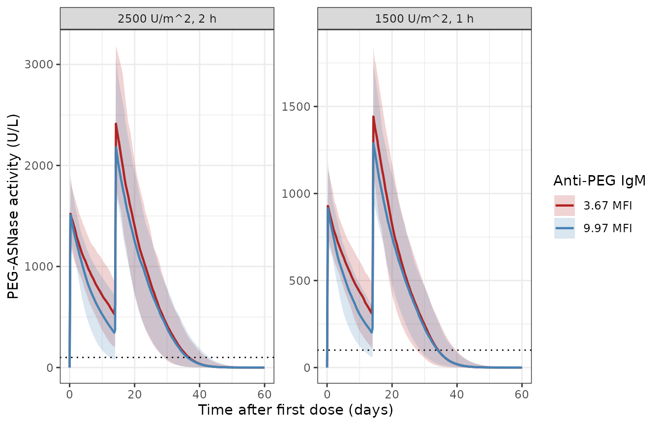
Simulated PEG-ASNase activity in induction: median (line) and 95% prediction interval (band), 200 patients per arm. Replicates Figure 4 of Siebel 2022 (a: 2500 U/m^2 over 2 h; b: 1500 U/m^2 over 1 h). Dotted line: 100 U/L.
fig4_trough <- fig4 |>
  filter(time == 13.999) |>
  group_by(arm) |>
  summarise(sim_median = median(Cc), sim_q25 = quantile(Cc, 0.25),
            sim_q75 = quantile(Cc, 0.75), sim_below_100 = 100 * mean(Cc < 100),
            .groups = "drop") |>
  left_join(arms, by = "arm") |>
  mutate(pct_diff_median = 100 * (sim_median - median) / median,
         pct_diff_q25 = 100 * (sim_q25 - q25) / q25,
         pct_diff_q75 = 100 * (sim_q75 - q75) / q75)

fig4_trough |>
  transmute(regimen, igm = sprintf("%.2f", igm),
            published = sprintf("%.0f (%.0f-%.0f)", median, q25, q75),
            simulated = sprintf("%.0f (%.0f-%.0f)", sim_median, sim_q25, sim_q75),
            pct_diff_median, pct_below_100, sim_below_100) |>
  dplyr::rename(
    "Regimen" = regimen,
    "Anti-PEG IgM (MFI)" = igm,
    "Published median (IQR), U/L" = published,
    "Simulated median (IQR), U/L" = simulated,
    "Median difference (%)" = pct_diff_median,
    "Published < 100 U/L (%)" = pct_below_100,
    "Simulated < 100 U/L (%)" = sim_below_100
  ) |>
knitr::kable(digits = 1, caption = "Day-14 trough after the first induction dose. Published values from Section 3.3 and ESM Table S5.")| Regimen | Anti-PEG IgM (MFI) | Published median (IQR), U/L | Simulated median (IQR), U/L | Median difference (%) | Published < 100 U/L (%) | Simulated < 100 U/L (%) |
|---|---|---|---|---|---|---|
| 2500 U/m^2, 2 h | 3.67 | 517 (391-632) | 521 (377-648) | 0.8 | 0.5 | 0.5 |
| 2500 U/m^2, 2 h | 9.97 | 339 (222-457) | 333 (216-445) | -1.7 | 4.9 | 4.0 |
| 1500 U/m^2, 1 h | 3.67 | 305 (241-367) | 304 (245-375) | -0.4 | 1.7 | 2.5 |
| 1500 U/m^2, 1 h | 9.97 | 194 (135-262) | 196 (132-253) | 1.0 | 14.9 | 16.0 |
# Assert on the centre and on the quartiles, never on the tails: the share of
# patients below 100 U/L lives in the tail of a 200-patient cohort and is
# reported above without a gate.
stopifnot(
  abs(median(fig4_trough$pct_diff_median)) < 7,
  max(abs(fig4_trough$pct_diff_median)) < 15,
  max(abs(c(fig4_trough$pct_diff_q25, fig4_trough$pct_diff_q75))) < 20,
  # Structural ordering: at each regimen the high-IgM arm has the lower trough.
  all(fig4_trough$sim_median[fig4_trough$igm == 9.97] <
        fig4_trough$sim_median[fig4_trough$igm == 3.67])
)
PKNCA validation
PKNCA recomputes exposure over the first induction dosing interval
(0-14 days) for a small covariate lattice, grouped by IgM arm. Siebel
2022 reports no NCA table, so the reference is the closed-form
AUC(0-14) of each virtual patient’s own solved parameters.
For a dose into the head of the chain the amount in compartment
j is D * exp(-(ke + kt) t) (kt t)^j / j!, which
integrates to
D * kt^j / (ke + kt)^(j + 1) * pgamma((ke + kt) T, j + 1).
The closed form is for a bolus; the simulated 2-hour infusion shifts the
profile by about an hour, which changes AUC(0-14) by well
under 1%.
lattice <- tidyr::expand_grid(
  BSA = c(0.5, 0.65, 0.78, 1.0, 1.4),
  AGE = c(3, 5.13, 12),
  SEXF = c(0, 1)
) |>
  # Keep BSA and age plausibly paired (small children are young).
  filter(!(BSA <= 0.65 & AGE == 12), !(BSA >= 1.4 & AGE == 3))

nca_subj <- tidyr::expand_grid(lattice, ABPEG_IGM = c(1.37, 9.97)) |>
  mutate(id = row_number(),
         treatment = ifelse(ABPEG_IGM > 3.67, "IgM 9.97 MFI", "IgM 1.37 MFI (median)"),
         amt = 2500 * BSA)

nca_grid <- sort(unique(c(seq(0, 1, by = 0.02), seq(1, 14, by = 0.25))))
ev_nca <- lapply(seq_len(nrow(nca_subj)), function(i) {
  s <- nca_subj[i, ]
  e <- rxode2::et(amt = s$amt, dur = 2 / 24, cmt = "central") |>
    rxode2::et(nca_grid, cmt = "central") |>
    as.data.frame()
  e$id <- s$id
  e
}) |>
  bind_rows() |>
  left_join(select(nca_subj, id, BSA, AGE, SEXF, ABPEG_IGM, treatment), by = "id") |>
  mutate(OCC = 1)

sim_nca <- rxode2::rxSolve(mod0, ev_nca, returnType = "data.frame",
                           keep = "treatment")
#> ℹ omega/sigma items treated as zero: 'etalcl', 'etaiov_vc_1', 'etaiov_vc_2', 'etaiov_vc_3', 'etaiov_cl_1', 'etaiov_cl_2', 'etaiov_cl_3'
#> Warning: multi-subject simulation without without 'omega'

nca_conc <- sim_nca |>
  filter(!is.na(Cc)) |>
  transmute(id, time, Cc, treatment)
nca_dose <- nca_subj |>
  transmute(id, time = 0, amt, treatment)

conc_obj <- PKNCA::PKNCAconc(nca_conc, Cc ~ time | treatment + id,
                             concu = "U/L", timeu = "day")
dose_obj <- PKNCA::PKNCAdose(nca_dose, amt ~ time | treatment + id, doseu = "U")
intervals <- data.frame(start = 0, end = 14, cmax = TRUE, tmax = TRUE,
                        auclast = TRUE)
nca_res <- PKNCA::pk.nca(PKNCA::PKNCAdata(conc_obj, dose_obj, intervals = intervals))

as.data.frame(nca_res) |>
  group_by(treatment, PPTESTCD) |>
  summarise(median = median(PPORRES, na.rm = TRUE), .groups = "drop") |>
  tidyr::pivot_wider(names_from = PPTESTCD, values_from = median) |>
  dplyr::rename(
    "IgM arm" = treatment,
    "AUC0-14d (U*day/L)" = auclast,
    "Cmax (U/L)" = cmax,
    "Tmax (day)" = tmax
  ) |>
knitr::kable(digits = 2, caption = "PKNCA over the first induction dosing interval, median per IgM arm.")| IgM arm | AUC0-14d (U*day/L) | Cmax (U/L) | Tmax (day) |
|---|---|---|---|
| IgM 1.37 MFI (median) | 13268.67 | 1541.41 | 0.1 |
| IgM 9.97 MFI | 11150.58 | 1538.58 | 0.1 |
auc_cf_0T <- function(D, V, CL, Q, T = 14) {
  ke <- CL / V; kt <- Q / V; j <- 0:13
  D / V * sum(kt^j / (ke + kt)^(j + 1) * pgamma((ke + kt) * T, j + 1))
}
indiv <- sim_nca |>
  filter(time == 1) |>
  select(id, vc, cl, q) |>
  left_join(select(nca_subj, id, amt, treatment), by = "id") |>
  rowwise() |>
  mutate(auc_ref = auc_cf_0T(amt, vc, cl, q)) |>
  ungroup()

reference <- indiv |>
  group_by(treatment) |>
  summarise(PPORRES = median(auc_ref), .groups = "drop") |>
  mutate(PPTESTCD = "auclast")

cmp <- nlmixr2lib::ncaComparisonTable(
  simulated     = nca_res,
  reference     = reference,
  by            = "treatment",
  params        = "auclast",
  units         = c(auclast = "U*day/L"),
  tolerance_pct = 20
)
knitr::kable(cmp, caption = "PKNCA AUC(0-14 days) against the closed-form AUC of each virtual patient's solved parameters, median per IgM arm. * marks rows differing by >20%.")| NCA parameter | treatment | Reference | Simulated | % diff |
|---|---|---|---|---|
| AUClast (U*day/L) | IgM 1.37 MFI (median) | 13300 | 13300 | -0.2% |
| AUClast (U*day/L) | IgM 9.97 MFI | 11200 | 11200 | -0.1% |
per_subj <- as.data.frame(nca_res) |>
  filter(PPTESTCD == "auclast") |>
  select(id, auclast = PPORRES) |>
  left_join(indiv, by = "id") |>
  mutate(pct = 100 * (auclast - auc_ref) / auc_ref)
summary(per_subj$pct)
#>    Min. 1st Qu.  Median    Mean 3rd Qu.    Max.
#> -0.1777 -0.1685 -0.1501 -0.1499 -0.1315 -0.1209

stopifnot(
  # Same parameters on both sides; the gap is the 2-hour infusion versus the
  # bolus closed form plus trapezoid error, so a tight bound is correct.
  max(abs(per_subj$pct)) < 1.5,
  # The arm above the cut point has the lower median exposure.
  median(per_subj$auclast[per_subj$treatment == "IgM 9.97 MFI"]) <
    median(per_subj$auclast[per_subj$treatment != "IgM 9.97 MFI"])
)
Assumptions and deviations
-
Reference model versus final model. Table 3 prints
both the reference model (no antibody covariate, refitted to this data
set) and the final covariate model. Only the final model is packaged, as
for any base-versus-final model-development paper. The reference model
is a refit of the Wurthwein 2021 structure with no new covariate; its
largest departure from the final model is the
CLinitialchange at the second induction dose (-0.125 against -0.107), which the authors attribute partly to the antibody effect. -
V,CLinitialandQtrare absolute, not per square metre. The control stream multiplies nothing by BSA beyond the linear centred term; theL/m^2tags record the convention of quoting values “for a child with BSA = 1 m^2”.model()renormalises each BSA factor to 1 at BSA = 1 m^2 so theini()values are the printed numbers. The alternative reading suggested by the wording of Wurthwein 2021 fits the paper’s own simulations less well (see above). -
Log base. The antibody level is log-transformed
with the natural logarithm: the paper pairs 1.30 with 3.67 MFI and 2.30
with 9.97 MFI, and
exp(1.30) = 3.67,exp(2.30) = 9.97. -
Antibody level supplied per record. The control
stream’s
IGMPLOGis the level before the first dose of the current treatment phase. Because the coefficient is non-zero only at the first induction dose, only the pre-induction value affects predictions; users can supply it on every record. -
Omega scale. Table 3 gives IIV and IOV as
percentages. They are taken as log-normal CVs,
omega^2 = log(1 + CV^2), the same convention used for the Wurthwein 2025 models of the same group; withomega^2 = CV^2the variances would be 3-4% larger. -
NONMEM
$OMEGA BLOCK(1) SAMEhas no nlmixr2 equivalent, so occasions 2 and 3 carry their own etas with the variance fixed equal to the occasion-1 estimate. -
Compartment naming. The control stream names the
states
CENTRALandPERI2-PERI14. These are not classical peripheral compartments (no back-flow, one shared volume), so thetransit<n>chain prefix is used. -
OCCcarries the phase effects, the IOV and the antibody gate. This is the authors’ own encoding. Occasion codes are renumbered from2/3/5to1..3. -
Simulation settings. The published simulations do
not state whether residual error was included; the replication above
uses the individual prediction
Ccwithout residual error. It uses 200 rather than 1000 patients per arm to keep the article fast to build. - Silent inactivation and hypersensitivity are out of scope. Records at or after either were excluded before fitting.
-
Screened but not retained: anti-PEG IgG (weaker
than IgM and uninformative once IgM is in the model) and all post-dose
antibody levels. They are listed in
covariatesDataExcluded.
Reference
Siebel C, Lanvers-Kaminsky C, Alten J, Smisek P, Nath CE, Rizzari C, Boos J, Wurthwein G. Impact of Antibodies Against Polyethylene Glycol on the Pharmacokinetics of PEGylated Asparaginase in Children with Acute Lymphoblastic Leukaemia: A Population Pharmacokinetic Approach. Eur J Drug Metab Pharmacokinet. 2022;47(2):187-198. https://doi.org/10.1007/s13318-021-00741-w