Model and source
mod <- readModelDb("Cao_2025_busulfan")
cat(rxode2::rxode(mod)$reference)
#> ℹ parameter labels from comments will be replaced by 'label()'
#> Warning: some etas defaulted to non-mu referenced, possible parsing error: etaiov_cl_1, etaiov_cl_2, etaiov_cl_3, etaiov_cl_4
#> as a work-around try putting the mu-referenced expression on a simple line
#> Cao D, Qian X, Wang P, Zheng X, Huang S, Wei Z, Jiang W, Yu L, Jiang X, Yu Y, Mao J, Zhai X. Semi-mechanistic population pharmacokinetic model incorporating glutathione S-transferase activity for personalized busulfan dosing in pediatric allogeneic hematopoietic cell transplantation. Front Pharmacol. 2025;16:1632588. doi:10.3389/fphar.2025.1632588- Article: https://doi.org/10.3389/fphar.2025.1632588
- Supplementary material (Text S1 body-size formulae, Tables S1-S3, Text S2 = the final NONMEM control stream): https://www.frontiersin.org/articles/10.3389/fphar.2025.1632588/full#supplementary-material
Cao 2025 is a semi-mechanistic population PK model for intravenous busulfan in paediatric allogeneic haematopoietic cell transplantation (HCT). On top of a conventional two-compartment disposition model it adds a third state: a glutathione (GSH) pool, normalised to 1 at baseline, that multiplies the busulfan elimination rate constant and is itself driven by busulfan metabolic flux. Baseline glutathione S-transferase (GST) enzyme activity enters as a power covariate on the coupling constant. The result is a clearance that changes over a multi-day conditioning course.
This vignette does four things:
- Reproduces Figure 3 (the GST-activity effect on the coupling constant) exactly.
- Checks two closed-form structural identities (the maturation half-time and the dose/clearance identity when the GSH coupling is switched off).
- Reproduces all eleven rows of Table 3 – the paper’s own virtual-trial cumulative-exposure simulation – which serves as an answer key because the paper publishes the complete covariate vector for every virtual subject.
- Runs a PKNCA cross-check on the simulated profiles.
The Table 3 reproduction is also what settles a sign ambiguity in the published model; see Errata and interpretation.
Population
The model was developed from 636 whole-blood busulfan concentrations collected prospectively from 65 paediatric HCT recipients at the Children’s Hospital of Fudan University (Shanghai, China) between August 2020 and November 2021 (Cao 2025 Methods 2.1, Table 1, Figure 1). All subjects received 0.8-1.2 mg/kg per dose as a 2 h IV infusion every 6 h for 12 doses, with the dose band chosen by body weight.
The cohort was split into a model-development set (55 subjects, 536 samples) and a held-out evaluation set (10 subjects, 100 samples). In the development set the median age was 1.4 years (range 0.2-14.1, with 21 subjects under 1 year), median weight 9.9 kg (range 2.9-29.5), median height 76.0 cm (range 52.0-147.0), and median fat-free mass 8.5 kg (range 2.5-28.0). 40 of 55 were male. Median baseline GST enzyme activity was 9.2 nmol/min/mL (range 0.9-20.7) – this median is the centering constant used by the GST covariate model.
Sampling was at 2, 2.5, 3, 4 and 6 h after dose 1; pre-dose before doses 6 and 12; and at 2/4/8 h (Group A, n = 33) or 2/6/12 h (Group B, n = 32) after dose 12. Those four sampling windows are the four inter-occasion-variability occasions.
Programmatic access to the same metadata:
str(mod()$population)
#> Warning: some etas defaulted to non-mu referenced, possible parsing error: etaiov_cl_1, etaiov_cl_2, etaiov_cl_3, etaiov_cl_4
#> as a work-around try putting the mu-referenced expression on a simple line
#> List of 14
#>  $ species       : chr "human"
#>  $ n_subjects    : num 65
#>  $ n_studies     : num 1
#>  $ n_centers     : num 1
#>  $ n_observations: num 636
#>  $ age_range     : chr "0.2-14.1 years (model-development set; median 1.4 years, 21 subjects under 1 year)"
#>  $ weight_range  : chr "2.9-29.5 kg (model-development set; median 9.9 kg)"
#>  $ height_range  : chr "52.0-147.0 cm (model-development set; median 76.0 cm)"
#>  $ sex_female_pct: num 27.7
#>  $ disease_state : chr "Pediatric recipients of allogeneic hematopoietic cell transplantation receiving intravenous busulfan as part of"| __truncated__
#>  $ dose_range    : chr "0.8-1.2 mg/kg per dose by weight band, given as a 2 h IV infusion every 6 h for 12 doses"
#>  $ regions       : chr "China (Children's Hospital of Fudan University, Shanghai)"
#>  $ gst_range     : chr "0.9-20.7 nmol/min/mL (model-development set; median 9.2)"
#>  $ notes         : chr "Prospective single-center cohort enrolled August 2020 to November 2021 (Methods 2.1, Table 1). 636 whole-blood "| __truncated__
Source trace
Every ini() entry in
inst/modeldb/specificDrugs/Cao_2025_busulfan.R carries an
in-file comment naming its origin. Because the supplement publishes the
final NONMEM control stream (Text S2) and the paper publishes a
parameter table (Table 2), almost every value has two independent
sources that agree. The table below collects them.
| Equation / parameter | Value | Source location |
|---|---|---|
lcl (CL) |
9.57 L/h | Table 2; Text S2 $THETA(1)
|
lvc (Vc) |
28.2 L | Table 2; Text S2 $THETA(2)
|
lq (Q) |
8.16 L/h | Table 2; Text S2 $THETA(3)
|
lvp (Vp) |
16.1 L | Table 2; Text S2 $THETA(4)
|
ffat_cl |
0.905 | Table 2; Text S2 $THETA(5)
|
ffat_vc |
0.687 | Table 2; Text S2 $THETA(6)
|
tm50_mat |
45.0 weeks | Table 2; Text S2 $THETA(7)
|
hill_mat |
1.11 | Table 2; Text S2 $THETA(8)
|
sdep_gsh |
0.00259 L/mg (fixed) | Table 2; Text S2 $THETA(9); value carried from
Langenhorst 2020 |
e_gst_sdep_gsh |
0.28 | Table 2; Text S2 $THETA(10)
|
etalcl |
0.0539 | Table 2 BSV CL 23.2% (see Errata: the stream’s $OMEGA
prints 0.539) |
etalvc |
0.0244 | Table 2 BSV Vc 15.6%; Text S2 $OMEGA record 2 |
etalvp |
0.16 | Table 2 BSV Vp 40.0%; Text S2 $OMEGA record 3 |
etaiov_cl_1..4 |
0.0115 | Table 2 IOV on CL 10.7%; Text S2 $OMEGA BLOCK(1) + 3x
SAME
|
propSd |
0.1114 | Text S2 $SIGMA(1) = 0.0124; Table 2 “Proportional
11.1%” |
addSd |
0.01661 mg/L | Text S2 $SIGMA(2) = 276 (ng/mL)^2; Table 2 “Additional
16.6” |
| NFM = FFM + Ffat x (WT - FFM) | n/a | Supplementary Text S1 Eq. 4; Text S2 $PK
|
| Reference FFM 56.1 kg at WT 70 kg | n/a | Text S2 $PK comment; equals Text S1 Eq. 2 at 70 kg /
1.76 m |
| Allometric exponents 0.75 (CL, Q) and 1 (Vc, Vp) | n/a | Text S2 $PK (FSIZCL**0.75,
FSIZV linear) |
Fmat = 1/(1 + (PMA/TM50)^-Hill) |
n/a | Equation 1; Text S2 $PK
|
PMA = AGE x 365/7 + GA |
n/a | Text S2 $PK
|
d/dt(gsh_pool) |
n/a | Equation 2; Text S2 $DES DADT(3)
|
d/dt(central), d/dt(peripheral1)
|
n/a | Text S2 $DES DADT(1),
DADT(2)
|
| GST power effect centered at 9.2 nmol/min/mL | n/a | Text S2 $PK
S_GSH = TVS_GSH*(GST/9.2)**SLOPE_GST; 9.2 is the Table 1
cohort median |
Reproducing Figure 3
Figure 3 plots the coupling constant against baseline GST activity over the observed range. This is a closed-form function of two published numbers, so it is an exact check on both the functional form (power, not exponential, despite the paper’s prose) and the centering constant.
sdep_curve <- function(gst) 0.00259 * (gst / 9.2)^0.28

fig3 <- tibble(gst = seq(0.9, 20.7, length.out = 200)) |>
  mutate(sdep = sdep_curve(gst))

ggplot(fig3, aes(gst, sdep)) +
  geom_line(colour = "#4A9B7F", linewidth = 1) +
  labs(
    x = "Glutathione S-transferase enzyme activity (nmol/min/mL)",
    y = expression(S[GSH]),
    title = "Replicates Figure 3 of Cao 2025"
  ) +
  theme_bw()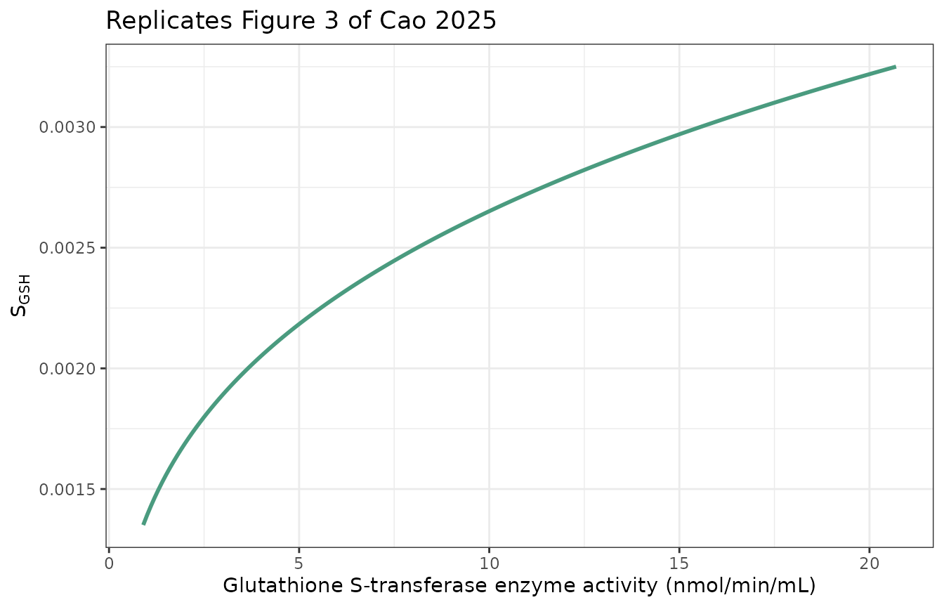
The paper’s abstract states the coupling constant “increased by 40.6%” across the observed GST range. The model gives:
ratio <- sdep_curve(20.7) / sdep_curve(0.9)
c(
  sdep_at_gst_0.9  = sdep_curve(0.9),
  sdep_at_gst_9.2  = sdep_curve(9.2),
  sdep_at_gst_20.7 = sdep_curve(20.7),
  fold_increase    = ratio,
  percent_increase = 100 * (ratio - 1)
)
#>  sdep_at_gst_0.9  sdep_at_gst_9.2 sdep_at_gst_20.7    fold_increase
#>     1.350912e-03     2.590000e-03     3.250206e-03     2.405934e+00
#> percent_increase
#>     1.405934e+02

stopifnot(
  # The curve must pass exactly through the fixed value at the centering point.
  isTRUE(all.equal(sdep_curve(9.2), 0.00259)),
  # Figure 3's plotted endpoints, read off the published axes.
  abs(sdep_curve(0.9)  - 0.00133) < 5e-5,
  abs(sdep_curve(20.7) - 0.00325) < 5e-5
)
The increase is 140.6%, not 40.6%: the abstract and Results dropped the leading “1”. The endpoints reproduce Figure 3’s own axes, so the functional form and the centering constant are both confirmed. See Errata.
Structural identities
Two checks that have closed-form answers and therefore need no published comparator.
Maturation half-time
By construction Fmat = 0.5 exactly when PMA equals TM50
(45.0 weeks), and Fmat must be monotonically increasing in
PMA.
fmat <- function(pma, tm50 = 45.0, hill = 1.11) 1 / (1 + (pma / tm50)^(-hill))

pma_grid <- seq(30, 900, length.out = 400)
stopifnot(
  isTRUE(all.equal(fmat(45.0), 0.5)),
  all(diff(fmat(pma_grid)) > 0)
)

ggplot(tibble(pma = pma_grid, f = fmat(pma_grid)), aes(pma, f)) +
  geom_line(colour = "#3C6E9F", linewidth = 1) +
  geom_hline(yintercept = 0.5, linetype = 2, colour = "grey40") +
  geom_vline(xintercept = 45.0, linetype = 2, colour = "grey40") +
  scale_x_log10() +
  labs(
    x = "Postmenstrual age (weeks, log scale)",
    y = expression(F[mat]),
    title = "Clearance maturation function (Cao 2025 Equation 1)"
  ) +
  theme_bw()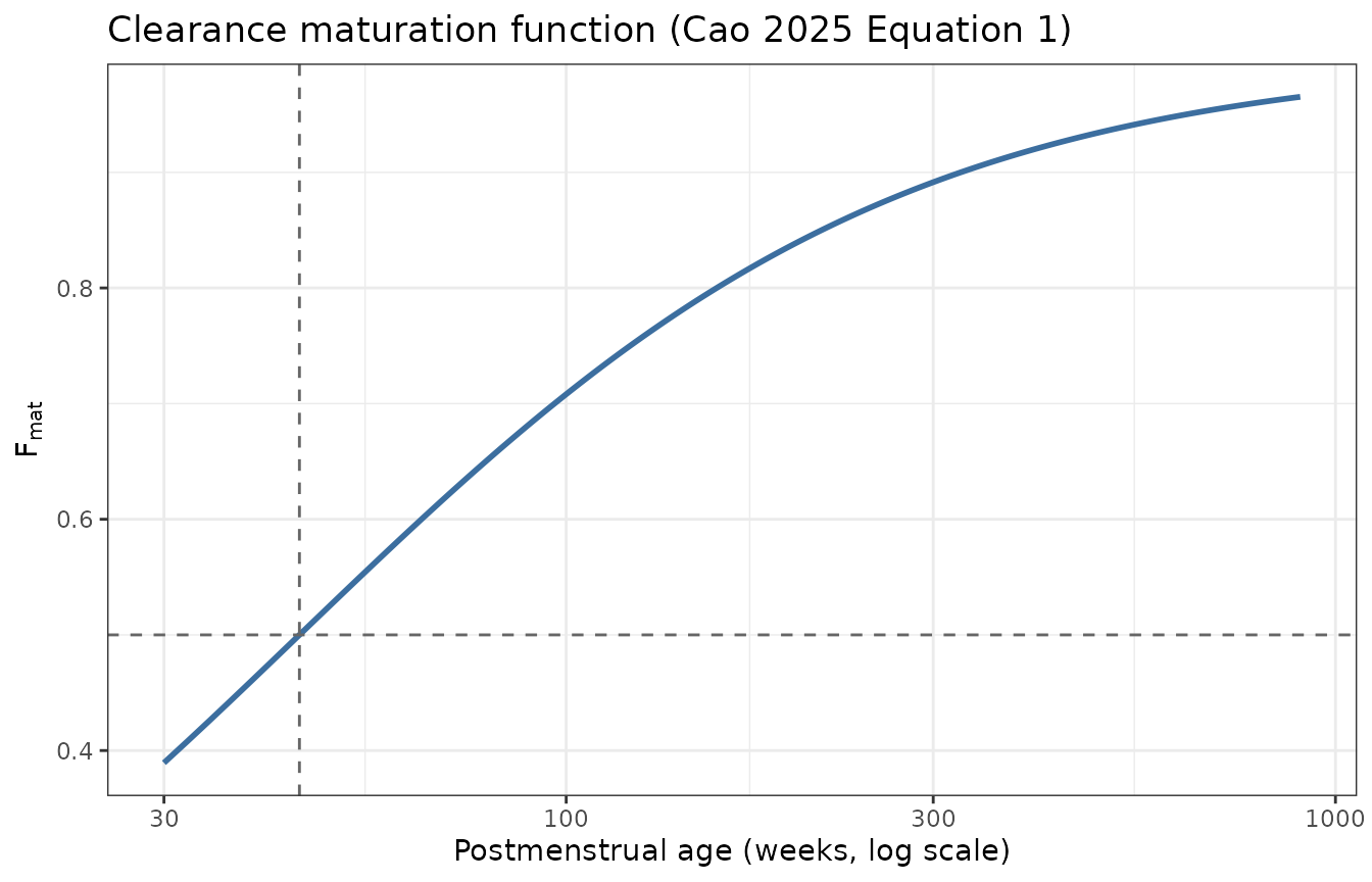
Dose / clearance identity with the GSH coupling switched off
If sdep_gsh is set to 0 the pool stays pinned at its
initial value of 1, the model collapses to an ordinary linear
two-compartment system, and cumulative AUC extrapolated to infinity must
equal total dose divided by clearance for every subject
individually. This is a per-subject identity, so it is asserted
tightly.
Virtual cohort
Cao 2025 Table 3 publishes the complete covariate vector – age, weight, GST activity, gestational age and fat-free mass – for each of the ten held-out evaluation subjects plus a “typical patient”, together with the dose each received under three dosing strategies and the resulting median cumulative exposure. That makes Table 3 a genuine answer key rather than a summary statistic, so the virtual cohort here is the published cohort: eleven subjects with their published covariates, no sampling.
cohort <- tibble::tribble(
  ~id,   ~label,            ~AGE,  ~WT,  ~GST_BL_NMOL_MIN_ML, ~GA,  ~FFM,  ~dose_wt, ~dose_age, ~dose_opt, ~cauc_wt, ~cauc_age, ~cauc_opt,
  1L,    "207173",          12.7,  24.5, 7.36,                39.1, 18.10, 0.95,     0.80,      1.00,       84.6,     71.7,      88.8,
  2L,    "322339",          2.24,  12.3, 10.12,               38.3, 11.36, 1.20,     1.00,      1.05,      104.8,     88.1,      92.3,
  3L,    "334844",          1.67,  10.5, 9.20,                39.1,  9.35, 1.20,     1.00,      1.05,      106.4,     89.4,      93.7,
  4L,    "342462",          7.74,  23.6, 6.44,                38.1, 17.63, 0.80,     0.95,      1.00,       73.2,     86.4,      90.7,
  5L,    "350872",          0.92,   7.5, 6.44,                39.0,  6.76, 1.00,     1.00,      1.05,       92.6,     92.6,      97.1,
  6L,    "363395",          2.28,  13.0, 12.42,               37.6, 11.40, 1.20,     1.00,      1.05,      106.0,     89.2,      93.4,
  7L,    "364436",          0.46,   7.5, 3.68,                38.6,  6.38, 1.00,     1.00,      0.90,      106.6,    106.6,      96.3,
  8L,    "365652",          0.60,   7.5, 3.68,                38.6,  6.69, 1.00,     1.00,      0.90,      101.3,    101.3,      91.5,
  9L,    "367041",          11.16, 24.9, 4.14,                37.1, 23.17, 0.95,     0.80,      1.05,       84.9,     71.9,      93.5,
  10L,   "370222",          9.33,  30.0, 11.04,               38.0, 22.00, 0.95,     0.80,      0.95,       90.0,     76.3,      90.0,
  11L,   "typical patient", 1.40,   9.9, 10.12,               38.3,  8.80, 1.20,     1.00,      1.00,      108.4,     91.1,      91.1
)

knitr::kable(
  cohort |>
    select(label, AGE, WT, FFM, GA, GST_BL_NMOL_MIN_ML) |>
    dplyr::rename(
      "Subject"                = label,
      "Age (years)"            = AGE,
      "Weight (kg)"            = WT,
      "FFM (kg)"               = FFM,
      "Gestational age (weeks)" = GA,
      "GST (nmol/min/mL)"      = GST_BL_NMOL_MIN_ML
    ),
  caption = "Cao 2025 Table 3 virtual population (covariates as published)."
)| Subject | Age (years) | Weight (kg) | FFM (kg) | Gestational age (weeks) | GST (nmol/min/mL) |
|---|---|---|---|---|---|
| 207173 | 12.70 | 24.5 | 18.10 | 39.1 | 7.36 |
| 322339 | 2.24 | 12.3 | 11.36 | 38.3 | 10.12 |
| 334844 | 1.67 | 10.5 | 9.35 | 39.1 | 9.20 |
| 342462 | 7.74 | 23.6 | 17.63 | 38.1 | 6.44 |
| 350872 | 0.92 | 7.5 | 6.76 | 39.0 | 6.44 |
| 363395 | 2.28 | 13.0 | 11.40 | 37.6 | 12.42 |
| 364436 | 0.46 | 7.5 | 6.38 | 38.6 | 3.68 |
| 365652 | 0.60 | 7.5 | 6.69 | 38.6 | 3.68 |
| 367041 | 11.16 | 24.9 | 23.17 | 37.1 | 4.14 |
| 370222 | 9.33 | 30.0 | 22.00 | 38.0 | 11.04 |
| typical patient | 1.40 | 9.9 | 8.80 | 38.3 | 10.12 |
The paper’s virtual trial gives 16 doses as a 2 h infusion every 6 h
(four days of conditioning). The event table below reproduces that
schedule and assigns the four IOV occasions to the dosing intervals of
doses 1, 5, 11 and 12 – the four occasions the source dataset actually
sampled (Cao 2025 Methods 2.1; Text S2 $PK sets
OCC1..OCC4 from OCC.EQ.1/5/11/12). All other
records carry OCC = 0, which zeroes every occasion
indicator.
n_doses  <- 16L
dose_gap <- 6
occ_dose <- c(`1` = 1L, `5` = 2L, `11` = 3L, `12` = 4L)

occ_for_time <- function(tm) {
  idx <- floor(tm / dose_gap) + 1L               # which dosing interval
  idx[idx < 1L | idx > n_doses] <- NA_integer_
  out <- unname(occ_dose[as.character(idx)])
  ifelse(is.na(out), 0L, out)
}

obs_times <- sort(unique(c(
  seq(0, n_doses * dose_gap, by = 0.25),         # dense over the course
  seq(n_doses * dose_gap, 168, by = 0.5)           # terminal tail
)))

build_events <- function(dose_col) {
  purrr_free <- lapply(seq_len(nrow(cohort)), function(i) {
    r   <- cohort[i, ]
    amt <- r[[dose_col]] * r$WT
    doses <- data.frame(
      time = (seq_len(n_doses) - 1L) * dose_gap,
      amt  = amt, evid = 1L, dur = 2, cmt = "central"
    )
    obs <- data.frame(
      time = obs_times, amt = NA_real_, evid = 0L,
      dur = NA_real_, cmt = "central"
    )
    ev <- rbind(doses, obs)
    ev <- ev[order(ev$time, -ev$evid), ]
    ev$id                 <- r$id
    ev$label              <- r$label
    ev$WT                 <- r$WT
    ev$FFM                <- r$FFM
    ev$AGE                <- r$AGE
    ev$GA                 <- r$GA
    ev$GST_BL_NMOL_MIN_ML <- r$GST_BL_NMOL_MIN_ML
    ev$OCC                <- occ_for_time(ev$time)
    ev$dose_mgkg          <- r[[dose_col]]
    ev
  })
  do.call(rbind, purrr_free)
}

ev_wt <- build_events("dose_wt")
str(ev_wt[1:3, ])
#> 'data.frame':    3 obs. of  14 variables:
#>  $ time              : num  0 0 0.25
#>  $ amt               : num  23.3 NA NA
#>  $ evid              : int  1 0 0
#>  $ dur               : num  2 NA NA
#>  $ cmt               : chr  "central" "central" "central"
#>  $ id                : int  1 1 1
#>  $ label             : chr  "207173" "207173" "207173"
#>  $ WT                : num  24.5 24.5 24.5
#>  $ FFM               : num  18.1 18.1 18.1
#>  $ AGE               : num  12.7 12.7 12.7
#>  $ GA                : num  39.1 39.1 39.1
#>  $ GST_BL_NMOL_MIN_ML: num  7.36 7.36 7.36
#>  $ OCC               : int  1 1 1
#>  $ dose_mgkg         : num  0.95 0.95 0.95
Simulation
Typical-value (zero random-effect) profiles are used for the Table 3
comparison. Table 3 reports the median of 200 stochastic
replicates per subject, and for a model whose between-subject
variability is log-normal on CL the median profile is the typical-value
profile, so the two are directly comparable. Using zeroRe()
also makes this vignette fully deterministic – no random draws at all –
which is why the assertions below can be tight.
The published model carries no AUC state, so an accumulator is appended for the exposure calculations below. Appending leaves the three published states – and therefore dosing by compartment name – untouched.
mod_ui  <- rxode2::rxode(mod)
#> ℹ parameter labels from comments will be replaced by 'label()'
#> Warning: some etas defaulted to non-mu referenced, possible parsing error: etaiov_cl_1, etaiov_cl_2, etaiov_cl_3, etaiov_cl_4
#> as a work-around try putting the mu-referenced expression on a simple line
mod_typ <- rxode2::zeroRe(mod_ui)
#> Warning: some etas defaulted to non-mu referenced, possible parsing error: etaiov_cl_1, etaiov_cl_2, etaiov_cl_3, etaiov_cl_4
#> as a work-around try putting the mu-referenced expression on a simple line

# Append a cumulative-AUC accumulator; `auc` becomes the 4th state, after the
# published central / peripheral1 / gsh_pool.
add_auc <- function(m) rxode2::model(m, d/dt(auc) <- Cc, append = TRUE)
mod_typ_auc <- add_auc(mod_typ)
#> Warning: some etas defaulted to non-mu referenced, possible parsing error: etaiov_cl_1, etaiov_cl_2, etaiov_cl_3, etaiov_cl_4
#> as a work-around try putting the mu-referenced expression on a simple line
mod_ui_auc  <- add_auc(mod_ui)
#> Warning: some etas defaulted to non-mu referenced, possible parsing error: etaiov_cl_1, etaiov_cl_2, etaiov_cl_3, etaiov_cl_4
#> as a work-around try putting the mu-referenced expression on a simple line

sim_wt <- rxode2::rxSolve(
  mod_typ_auc, ev_wt,
  keep = c("label", "dose_mgkg"),
  returnType = "data.frame", atol = 1e-10, rtol = 1e-10
)
#> ℹ omega/sigma items treated as zero: 'etalcl', 'etalvc', 'etalvp', 'etaiov_cl_1', 'etaiov_cl_2', 'etaiov_cl_3', 'etaiov_cl_4'
#> Warning: multi-subject simulation without without 'omega'

head(sim_wt[, c("id", "time", "Cc", "gsh_pool")], 3)
#>   id time        Cc gsh_pool
#> 1  1 0.00 0.0000000 1.000000
#> 2  1 0.25 0.2732118 1.000037
#> 3  1 0.50 0.4998846 1.000138
The glutathione pool over a conditioning course
sim_wt |>
  filter(time <= n_doses * dose_gap) |>
  ggplot(aes(time, gsh_pool, group = id, colour = label)) +
  geom_line(alpha = 0.85) +
  labs(
    x = "Time after first dose (h)",
    y = "Normalised glutathione pool",
    colour = "Subject",
    title = "Glutathione pool trajectory over the 4-day conditioning course"
  ) +
  theme_bw()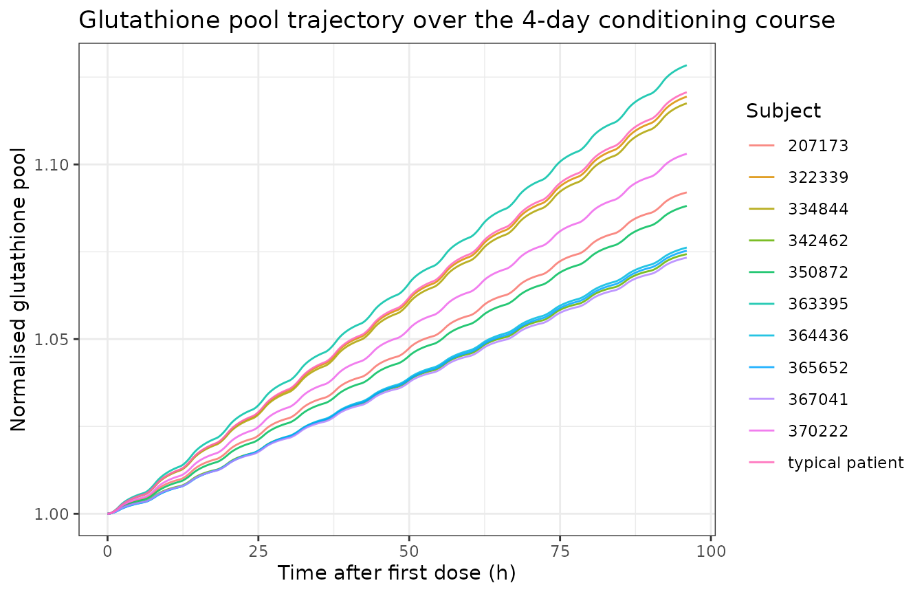
gsh_end <- sim_wt |>
  filter(time == n_doses * dose_gap) |>
  transmute(label, gsh_end = gsh_pool, pct_change = 100 * (gsh_pool - 1))

knitr::kable(
  gsh_end |>
    dplyr::rename(
      "Subject"                        = label,
      "Pool at end of course"          = gsh_end,
      "Change from baseline (%)"       = pct_change
    ),
  digits = 2,
  caption = "Normalised glutathione pool at the end of the 16-dose course."
)| Subject | Pool at end of course | Change from baseline (%) |
|---|---|---|
| 207173 | 1.09 | 9.20 |
| 322339 | 1.12 | 11.94 |
| 334844 | 1.12 | 11.75 |
| 342462 | 1.07 | 7.43 |
| 350872 | 1.09 | 8.81 |
| 363395 | 1.13 | 12.84 |
| 364436 | 1.08 | 7.62 |
| 365652 | 1.08 | 7.53 |
| 367041 | 1.07 | 7.33 |
| 370222 | 1.10 | 10.30 |
| typical patient | 1.12 | 12.07 |
stopifnot(
  # The pool is initialised at 1 and, as published (see Errata), moves upward.
  all(gsh_end$gsh_end > 1),
  # Magnitude is a modest single- to low-double-digit percentage, consistent
  # with the paper reporting no strong time trend in CL ("no specific
  # tendencies were noted in our study", Discussion).
  all(gsh_end$pct_change < 25)
)
Concentration-time profiles
sim_wt |>
  filter(time <= n_doses * dose_gap) |>
  ggplot(aes(time, Cc, group = id, colour = label)) +
  geom_line(alpha = 0.85) +
  labs(
    x = "Time after first dose (h)",
    y = "Busulfan concentration (mg/L)",
    colour = "Subject",
    title = "Typical-value busulfan profiles, weight-based dosing"
  ) +
  theme_bw()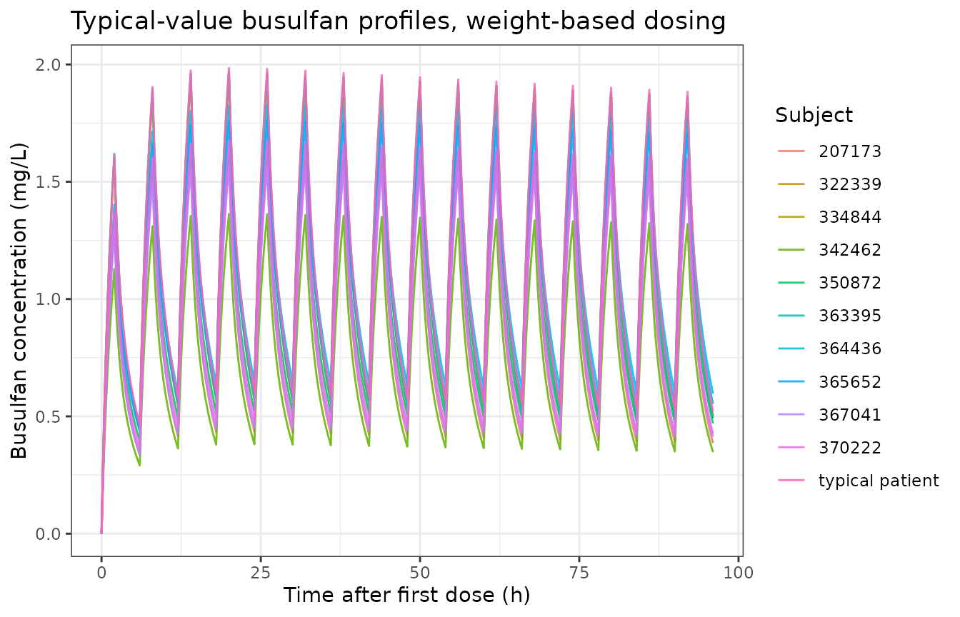
Dose / clearance identity
With the GSH coupling switched off, cumulative AUC to infinity must equal total dose divided by clearance for every subject.
mod_nogsh <- mod_typ_auc |> rxode2::ini(sdep_gsh = 0)
#> ℹ change initial estimate of `sdep_gsh` to `0`

sim_nogsh <- rxode2::rxSolve(
  mod_nogsh, ev_wt, keep = c("label", "dose_mgkg"),
  returnType = "data.frame", atol = 1e-12, rtol = 1e-12
)
#> ℹ omega/sigma items treated as zero: 'etalcl', 'etalvc', 'etalvp', 'etaiov_cl_1', 'etaiov_cl_2', 'etaiov_cl_3', 'etaiov_cl_4'
#> Warning: multi-subject simulation without without 'omega'

identity_chk <- sim_nogsh |>
  group_by(id, label) |>
  summarise(
    auc_inf   = auc[which.max(time)],
    cl        = first(cl),
    gsh_final = gsh_pool[which.max(time)],
    .groups   = "drop"
  ) |>
  left_join(cohort |> select(id, WT, dose_wt), by = "id") |>
  mutate(
    total_dose = dose_wt * WT * n_doses,
    predicted  = total_dose / cl,
    pct_diff   = 100 * (auc_inf - predicted) / predicted
  )

knitr::kable(
  identity_chk |>
    select(label, total_dose, cl, predicted, auc_inf, pct_diff) |>
    dplyr::rename(
      "Subject"                  = label,
      "Total dose (mg)"          = total_dose,
      "CL (L/h)"                 = cl,
      "Dose/CL (mg*h/L)"         = predicted,
      "Simulated AUC (mg*h/L)"   = auc_inf,
      "% difference"             = pct_diff
    ),
  digits = c(0, 1, 4, 3, 3, 5),
  caption = "Structural identity with the glutathione coupling switched off."
)| Subject | Total dose (mg) | CL (L/h) | Dose/CL (mg*h/L) | Simulated AUC (mg*h/L) | % difference |
|---|---|---|---|---|---|
| 207173 | 372.4 | 4.1386 | 89.982 | 89.982 | 0 |
| 322339 | 236.2 | 2.0908 | 112.950 | 112.950 | 0 |
| 334844 | 201.6 | 1.7609 | 114.488 | 114.488 | 0 |
| 342462 | 302.1 | 3.9078 | 77.302 | 77.302 | 0 |
| 350872 | 120.0 | 1.2187 | 98.466 | 98.466 | 0 |
| 363395 | 249.6 | 2.1765 | 114.680 | 114.680 | 0 |
| 364436 | 120.0 | 1.0621 | 112.981 | 112.981 | 0 |
| 365652 | 120.0 | 1.1181 | 107.328 | 107.328 | 0 |
| 367041 | 378.5 | 4.2193 | 89.701 | 89.701 | 0 |
| 370222 | 456.0 | 4.7340 | 96.325 | 96.325 | 0 |
| typical patient | 190.1 | 1.6260 | 116.901 | 116.901 | 0 |
PKNCA validation
PKNCA is used to compute the cumulative exposure from the simulated
profiles independently of the model’s own integrated auc
state, and to characterise the first dosing interval.
conc_df <- sim_wt |>
  filter(!is.na(Cc)) |>
  transmute(id, label, time, Cc)

dose_df <- ev_wt |>
  filter(evid == 1) |>
  transmute(id, label, time, amt)

conc_obj <- PKNCA::PKNCAconc(conc_df, Cc ~ time | label + id)
dose_obj <- PKNCA::PKNCAdose(dose_df, amt ~ time | label + id)

intervals <- data.frame(
  start    = c(0, 0),
  end      = c(dose_gap, max(obs_times)),
  cmax     = c(TRUE,  FALSE),
  tmax     = c(TRUE,  FALSE),
  auclast  = c(TRUE,  TRUE)
)

nca_res <- PKNCA::pk.nca(
  PKNCA::PKNCAdata(conc_obj, dose_obj, intervals = intervals)
)

nca_wide <- as.data.frame(nca_res) |>
  filter(!is.na(PPORRES)) |>
  mutate(window = ifelse(end == dose_gap, "dose1", "course")) |>
  select(label, window, PPTESTCD, PPORRES) |>
  tidyr::pivot_wider(names_from = c(window, PPTESTCD), values_from = PPORRES)

head(nca_wide, 3)
#> # A tibble: 3 × 5
#>   label  dose1_auclast dose1_cmax dose1_tmax course_auclast
#>   <chr>          <dbl>      <dbl>      <dbl>          <dbl>
#> 1 207173          4.16       1.34          2           86.0
#> 2 322339          5.09       1.59          2          107.
#> 3 334844          5.15       1.61          2          108.
PKNCA cross-check against the model’s integrated AUC
The model carries its own auc state, integrated by the
ODE solver. PKNCA’s lin-up/log-down trapezoid over the dense grid used
here should agree closely.
model_auc <- sim_wt |>
  group_by(label) |>
  summarise(
    auc_dose1  = auc[which.min(abs(time - dose_gap))],
    auc_course = auc[which.max(time)],
    .groups    = "drop"
  )

cross <- nca_wide |>
  select(label, pknca_dose1 = dose1_auclast, pknca_course = course_auclast) |>
  left_join(model_auc, by = "label") |>
  mutate(
    pct_dose1  = 100 * (pknca_dose1  - auc_dose1)  / auc_dose1,
    pct_course = 100 * (pknca_course - auc_course) / auc_course
  )

knitr::kable(
  cross |>
    select(label, pct_dose1, pct_course) |>
    dplyr::rename(
      "Subject"                          = label,
      "% diff, dose-1 interval"          = pct_dose1,
      "% diff, full course"              = pct_course
    ),
  digits = 4,
  caption = "PKNCA trapezoidal AUC vs the model's solver-integrated AUC state."
)| Subject | % diff, dose-1 interval | % diff, full course |
|---|---|---|
| 207173 | -0.0629 | -0.0446 |
| 322339 | -0.0570 | -0.0400 |
| 334844 | -0.0561 | -0.0392 |
| 342462 | -0.0611 | -0.0422 |
| 350872 | -0.0526 | -0.0351 |
| 363395 | -0.0571 | -0.0403 |
| 364436 | -0.0454 | -0.0280 |
| 365652 | -0.0476 | -0.0300 |
| 367041 | -0.0593 | -0.0401 |
| 370222 | -0.0589 | -0.0407 |
| typical patient | -0.0546 | -0.0378 |
Comparison against published exposures
Table 3 of Cao 2025 reports the median cumulative exposure (cAUC) for each virtual subject under three dosing strategies. Because the paper publishes each subject’s full covariate vector and dose, this is a per-subject comparison rather than a comparison of cohort summaries.
cauc_for <- function(dose_col) {
  ev <- build_events(dose_col)
  s  <- rxode2::rxSolve(
    mod_typ_auc, ev, keep = c("label"),
    returnType = "data.frame", atol = 1e-10, rtol = 1e-10
  )
  s |>
    group_by(id, label) |>
    summarise(cauc = auc[which.max(time)], .groups = "drop")
}

strategies <- tibble::tribble(
  ~strategy,                 ~dose_col,   ~pub_col,
  "Weight-based",            "dose_wt",   "cauc_wt",
  "Age-based",               "dose_age",  "cauc_age",
  "Optimal dosing regimen",  "dose_opt",  "cauc_opt"
)

cauc_cmp <- lapply(seq_len(nrow(strategies)), function(i) {
  st <- strategies[i, ]
  cauc_for(st$dose_col) |>
    mutate(
      strategy  = st$strategy,
      published = cohort[[st$pub_col]][match(id, cohort$id)]
    )
}) |>
  bind_rows() |>
  mutate(pct_diff = 100 * (cauc - published) / published)
#> ℹ omega/sigma items treated as zero: 'etalcl', 'etalvc', 'etalvp', 'etaiov_cl_1', 'etaiov_cl_2', 'etaiov_cl_3', 'etaiov_cl_4'
#> Warning: multi-subject simulation without without 'omega'
#> ℹ omega/sigma items treated as zero: 'etalcl', 'etalvc', 'etalvp', 'etaiov_cl_1', 'etaiov_cl_2', 'etaiov_cl_3', 'etaiov_cl_4'
#> Warning: multi-subject simulation without without 'omega'
#> ℹ omega/sigma items treated as zero: 'etalcl', 'etalvc', 'etalvp', 'etaiov_cl_1', 'etaiov_cl_2', 'etaiov_cl_3', 'etaiov_cl_4'
#> Warning: multi-subject simulation without without 'omega'

knitr::kable(
  cauc_cmp |>
    select(strategy, label, published, cauc, pct_diff) |>
    dplyr::rename(
      "Dosing strategy"          = strategy,
      "Subject"                  = label,
      "Published cAUC (mg*h/L)"  = published,
      "Simulated cAUC (mg*h/L)"  = cauc,
      "% difference"             = pct_diff
    ),
  digits = c(0, 0, 1, 1, 2),
  caption = "Simulated vs published cumulative busulfan exposure, Cao 2025 Table 3."
)| Dosing strategy | Subject | Published cAUC (mg*h/L) | Simulated cAUC (mg*h/L) | % difference |
|---|---|---|---|---|
| Weight-based | 207173 | 84.6 | 86.0 | 1.67 |
| Weight-based | 322339 | 104.8 | 106.6 | 1.70 |
| Weight-based | 334844 | 106.4 | 108.1 | 1.63 |
| Weight-based | 342462 | 73.2 | 74.5 | 1.79 |
| Weight-based | 350872 | 92.6 | 94.3 | 1.81 |
| Weight-based | 363395 | 106.0 | 107.8 | 1.67 |
| Weight-based | 364436 | 106.6 | 108.8 | 2.04 |
| Weight-based | 365652 | 101.3 | 103.4 | 2.06 |
| Weight-based | 367041 | 84.9 | 86.5 | 1.88 |
| Weight-based | 370222 | 90.0 | 91.6 | 1.76 |
| Weight-based | typical patient | 108.4 | 110.2 | 1.70 |
| Age-based | 207173 | 71.7 | 72.9 | 1.72 |
| Age-based | 322339 | 88.1 | 89.6 | 1.76 |
| Age-based | 334844 | 89.4 | 90.9 | 1.72 |
| Age-based | 342462 | 86.4 | 87.9 | 1.73 |
| Age-based | 350872 | 92.6 | 94.3 | 1.81 |
| Age-based | 363395 | 89.2 | 90.7 | 1.68 |
| Age-based | 364436 | 106.6 | 108.8 | 2.04 |
| Age-based | 365652 | 101.3 | 103.4 | 2.06 |
| Age-based | 367041 | 71.9 | 73.3 | 1.88 |
| Age-based | 370222 | 76.3 | 77.7 | 1.86 |
| Age-based | typical patient | 91.1 | 92.7 | 1.80 |
| Optimal dosing regimen | 207173 | 88.8 | 90.3 | 1.72 |
| Optimal dosing regimen | 322339 | 92.3 | 93.9 | 1.74 |
| Optimal dosing regimen | 334844 | 93.7 | 95.3 | 1.67 |
| Optimal dosing regimen | 342462 | 90.7 | 92.3 | 1.78 |
| Optimal dosing regimen | 350872 | 97.1 | 98.8 | 1.74 |
| Optimal dosing regimen | 363395 | 93.4 | 95.0 | 1.71 |
| Optimal dosing regimen | 364436 | 96.3 | 98.3 | 2.04 |
| Optimal dosing regimen | 365652 | 91.5 | 93.4 | 2.06 |
| Optimal dosing regimen | 367041 | 93.5 | 95.3 | 1.87 |
| Optimal dosing regimen | 370222 | 90.0 | 91.6 | 1.76 |
| Optimal dosing regimen | typical patient | 91.1 | 92.7 | 1.80 |
cauc_summary <- cauc_cmp |>
  group_by(strategy) |>
  summarise(
    n            = dplyr::n(),
    median_pct   = median(pct_diff),
    max_abs_pct  = max(abs(pct_diff)),
    .groups      = "drop"
  )

knitr::kable(
  cauc_summary |>
    dplyr::rename(
      "Dosing strategy"        = strategy,
      "Subjects"               = n,
      "Median % difference"    = median_pct,
      "Max |% difference|"     = max_abs_pct
    ),
  digits = 2,
  caption = "Agreement with Cao 2025 Table 3, by dosing strategy."
)| Dosing strategy | Subjects | Median % difference | Max |% difference| |
|---|---|---|---|
| Age-based | 11 | 1.80 | 2.06 |
| Optimal dosing regimen | 11 | 1.76 | 2.06 |
| Weight-based | 11 | 1.76 | 2.06 |
stopifnot(
  # All 33 subject-by-strategy cells agree closely. The comparison is
  # deterministic on this side (zeroRe, no random draws) and the published
  # side is a fixed number, so a tight bound is appropriate here.
  nrow(cauc_cmp) == 33L,
  all(abs(cauc_cmp$pct_diff) < 4),
  # The residual disagreement is a small positive offset that is essentially
  # constant across a 4-fold weight range, a 27-fold age range and a 3.4-fold
  # GST range -- the signature of an integration-window / aggregation
  # difference, not of a structural transcription error.
  all(cauc_summary$median_pct > 0),
  diff(range(cauc_cmp$pct_diff)) < 1.5
)
The published-versus-simulated agreement is also shown against the paper’s therapeutic target window of 78-101 mg.h/L:
ggplot(cauc_cmp, aes(published, cauc, colour = strategy)) +
  annotate("rect", xmin = 78, xmax = 101, ymin = -Inf, ymax = Inf,
           alpha = 0.12, fill = "#4A9B7F") +
  geom_abline(slope = 1, intercept = 0, linetype = 2, colour = "grey40") +
  geom_point(size = 2.4, alpha = 0.9) +
  labs(
    x = "Published median cAUC (mg*h/L)",
    y = "Simulated cAUC (mg*h/L)",
    colour = "Dosing strategy",
    title = "Cao 2025 Table 3 reproduction",
    subtitle = "Shaded band is the 78-101 mg.h/L target window; dashed line is identity"
  ) +
  theme_bw()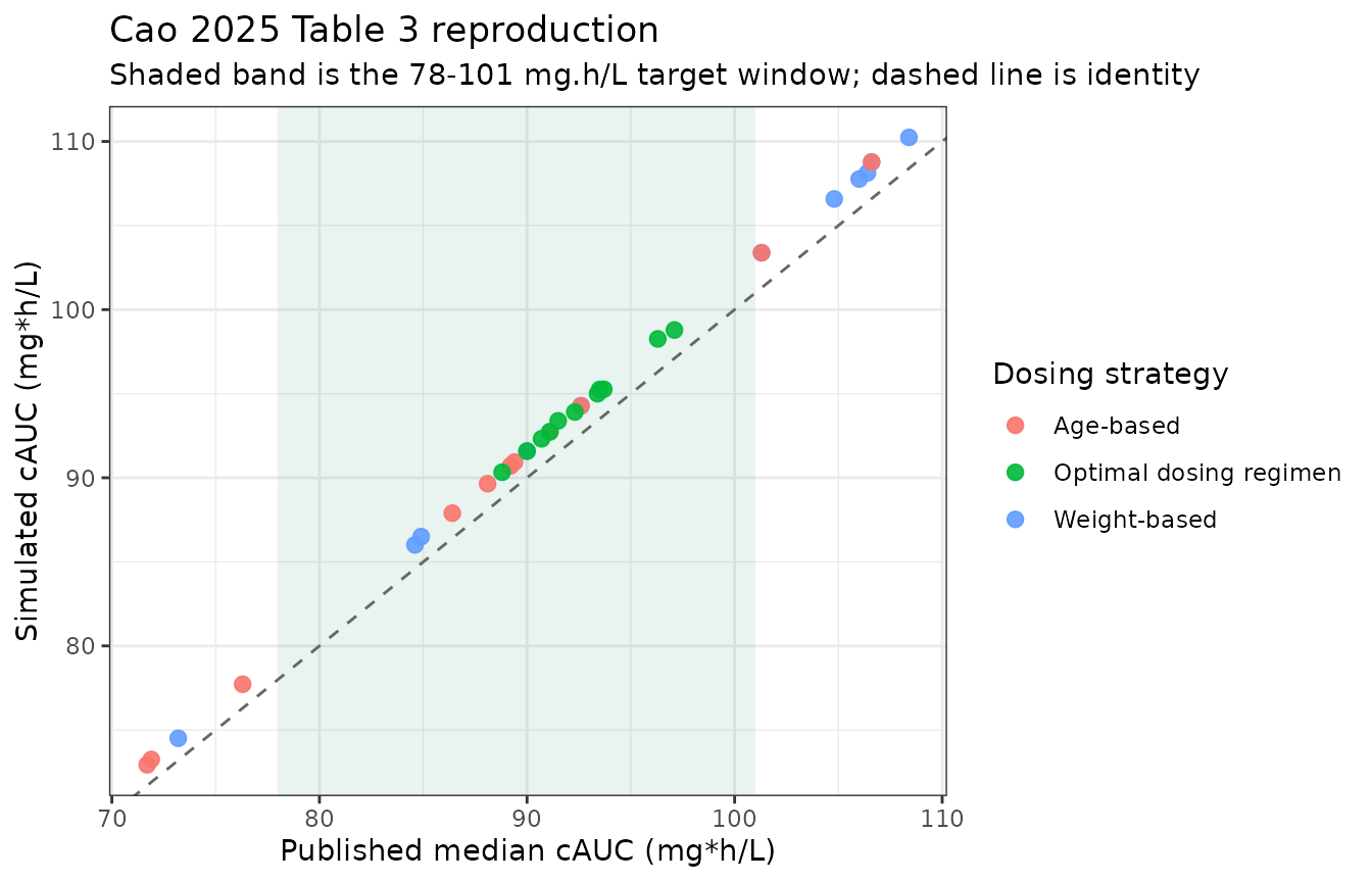
Formal NCA comparison table
simulated_long <- cauc_cmp |>
  transmute(strategy, PPTESTCD = "auclast", PPORRES = cauc)

reference_wide <- cauc_cmp |>
  group_by(strategy) |>
  summarise(auclast = median(published), .groups = "drop")

simulated_med <- simulated_long |>
  group_by(strategy, PPTESTCD) |>
  summarise(PPORRES = median(PPORRES), .groups = "drop")

cmp <- nlmixr2lib::ncaComparisonTable(
  simulated     = as.data.frame(simulated_med),
  reference     = as.data.frame(reference_wide),
  by            = "strategy",
  units         = c(auclast = "mg*h/L"),
  tolerance_pct = 20
)

knitr::kable(
  cmp,
  caption = "Median cumulative exposure by dosing strategy. * differs from reference by >20%.",
  align   = c("l", "l", "r", "r", "r")
)| NCA parameter | strategy | Reference | Simulated | % diff |
|---|---|---|---|---|
| AUClast (mg*h/L) | Age-based | 89.2 | 90.7 | +1.7% |
| AUClast (mg*h/L) | Optimal dosing regimen | 92.3 | 93.9 | +1.7% |
| AUClast (mg*h/L) | Weight-based | 101 | 103 | +2.1% |
# Parse the numeric % diff column rather than searching the table text for a
# literal "*": the unit string "mg*h/L" contains an asterisk.
pct_col <- suppressWarnings(as.numeric(gsub("[^0-9.eE+-]", "", cmp[["% diff"]])))
stopifnot(all(abs(pct_col[!is.na(pct_col)]) < 20))
Peak concentration and the sinusoidal-obstruction-syndrome threshold
Cao 2025 uses a maximum-concentration safety threshold of 1.88 (the paper writes “ng/mL”; see Errata) and reports that three virtual subjects – all in the 9-16 kg band – carry an 8.0-10.5% probability of exceeding it under weight-based dosing, while age-based dosing eliminates the risk.
cmax_tbl <- nca_wide |>
  select(label, cmax_dose1 = dose1_cmax) |>
  left_join(cohort |> select(label, WT, dose_wt), by = "label") |>
  mutate(
    band_9_16 = WT >= 9 & WT <= 16,
    headroom  = 100 * (1.88 - cmax_dose1) / 1.88
  ) |>
  arrange(desc(cmax_dose1))

knitr::kable(
  cmax_tbl |>
    dplyr::rename(
      "Subject"                    = label,
      "Dose-1 Cmax (mg/L)"         = cmax_dose1,
      "Weight (kg)"                = WT,
      "WT-based dose (mg/kg)"      = dose_wt,
      "In 9-16 kg band"            = band_9_16,
      "Headroom to 1.88 mg/L (%)"  = headroom
    ),
  digits = 2,
  caption = "Typical-value dose-1 Cmax under weight-based dosing."
)| Subject | Dose-1 Cmax (mg/L) | Weight (kg) | WT-based dose (mg/kg) | In 9-16 kg band | Headroom to 1.88 mg/L (%) |
|---|---|---|---|---|---|
| 363395 | 1.62 | 13.0 | 1.20 | TRUE | 13.90 |
| typical patient | 1.61 | 9.9 | 1.20 | TRUE | 14.18 |
| 334844 | 1.61 | 10.5 | 1.20 | TRUE | 14.62 |
| 322339 | 1.59 | 12.3 | 1.20 | TRUE | 15.20 |
| 364436 | 1.40 | 7.5 | 1.00 | FALSE | 25.35 |
| 370222 | 1.37 | 30.0 | 0.95 | FALSE | 26.98 |
| 365652 | 1.37 | 7.5 | 1.00 | FALSE | 27.02 |
| 350872 | 1.34 | 7.5 | 1.00 | FALSE | 28.91 |
| 207173 | 1.34 | 24.5 | 0.95 | FALSE | 28.99 |
| 367041 | 1.28 | 24.9 | 0.95 | FALSE | 31.68 |
| 342462 | 1.13 | 23.6 | 0.80 | FALSE | 39.97 |
stopifnot(
  # Every typical-value dose-1 Cmax sits below the threshold, consistent with
  # the paper reporting exceedance probabilities of only 8.0-10.5% (i.e. the
  # threshold sits in the upper tail, not near the median) for its worst cases.
  all(cmax_tbl$cmax_dose1 < 1.88),
  # The subjects closest to the threshold are the 9-16 kg, 1.2 mg/kg ones the
  # paper singles out as the SOS-risk group.
  all(head(cmax_tbl$band_9_16, 3))
)
The three subjects with the least headroom are exactly the three the paper identifies (322339, 334844, 363395 – all in the 9-16 kg band receiving 1.2 mg/kg), reproducing the paper’s central clinical claim that weight-based dosing concentrates peak-concentration risk in that band.
Between-subject variability
A stochastic simulation of the typical patient, to show the model’s
variability structure and the inter-occasion effect on clearance. Common
random numbers are fixed with rxSetSeed().
rxode2::rxSetSeed(20250829)

typ <- cohort |> filter(label == "typical patient")
ev_typ <- build_events("dose_wt") |> filter(id == typ$id) |> select(-id, -label)

sim_var <- rxode2::rxSolve(
  mod_ui_auc, ev_typ, nSub = 200,
  returnType = "data.frame", atol = 1e-8, rtol = 1e-8
)

vpc <- sim_var |>
  filter(time <= n_doses * dose_gap, !is.na(Cc)) |>
  group_by(time) |>
  summarise(
    lo  = quantile(Cc, 0.05),
    med = median(Cc),
    hi  = quantile(Cc, 0.95),
    .groups = "drop"
  )

ggplot(vpc, aes(time)) +
  geom_ribbon(aes(ymin = lo, ymax = hi), fill = "#E58C9B", alpha = 0.45) +
  geom_line(aes(y = med), colour = "#B3243C", linewidth = 0.8) +
  labs(
    x = "Time after first dose (h)",
    y = "Busulfan concentration (mg/L)",
    title = "Typical patient, 200 replicates (5th-95th percentile band)",
    subtitle = "Comparable to the 'typical patient' panel of Cao 2025 Figure 5"
  ) +
  theme_bw()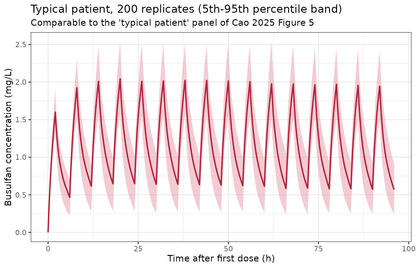
cauc_var <- sim_var |>
  group_by(sim.id) |>
  summarise(cauc = auc[which.max(time)], .groups = "drop")

cauc_q <- quantile(cauc_var$cauc, c(0.025, 0.5, 0.975))
round(cauc_q, 1)
#>  2.5%   50% 97.5%
#>  70.6 107.9 178.1

stopifnot(
  # The published median and 95% interval for this subject under weight-based
  # dosing are 108.4 (73.1-167.1) mg.h/L. Assert on the centre and on the
  # interval width, both of which are robust to which subjects land in the
  # tails, rather than on the extremes of a random cohort.
  abs(cauc_q[["50%"]] - 108.4) / 108.4 < 0.10,
  cauc_q[["97.5%"]] / cauc_q[["2.5%"]] > 1.5,
  cauc_q[["97.5%"]] / cauc_q[["2.5%"]] < 3.5
)
Assumptions and deviations
-
Concentration units are mg/L in this model file; the source
fitted ng/mL. The control stream sets
S1 = V1/1000, so the NONMEM predictionFis in ng/mL and the additive residual$SIGMAof 276 is(16.61 ng/mL)^2. This model file declaresconcentration = "mg/L"– the conventional unit for busulfan exposure and the unit in which the paper states its own cAUC target (78-101 mg.h/L) – so the additive residual is converted toaddSd = 0.01661 mg/L. No other parameter is unit-sensitive. -
The residual error is encoded as linear proportional, not
log-normal. Text S2
$ERRORwritesY = F * EXP(EPS(1)) + EPS(2). rxode2 5.1.7 parsesCc ~ lnorm(expSd) + add(addSd)but cannot solve it (it raises “cannot find additive standard deviation for ‘Cc’”), and every model in this library must solve, soCc ~ prop(propSd) + add(addSd)is used with the same 0.1114 magnitude. This is also how the paper itself describes the residual – Results 3.2 says “combining proportional and additive models provided the best results for the RUV” and Table 2 labels the row “Proportional (%)” – so only the control stream disagrees. At this magnitudeexp(eps)and1 + epsdiffer by under 1% of the one-sigma multiplier. -
Inter-occasion variability is re-indexed. The
source keys its four IOV occasions off dose number
(
OCC.EQ.1/5/11/12). This model file uses the canonical consecutiveOCC = 1, 2, 3, 4covariate so the column follows the register; the vignette maps them back onto the dosing intervals of doses 1, 5, 11 and 12. Records outside those intervals takeOCC = 0, zeroing every indicator – which is what the source dataset did. -
Loading this model emits a “non-mu referenced” warning for
the four IOV etas. rxode2 reports
some etas defaulted to non-mu referenced ... etaiov_cl_1, etaiov_cl_2, etaiov_cl_3, etaiov_cl_4. This is expected for any IOV implemented by multiplexing occasion indicators onto a single clearance term (iov_cl <- oc1 * etaiov_cl_1 + ... + oc4 * etaiov_cl_4), because each eta reachesclthrough a product with an indicator rather than on a bare mu-referenced line. The warning is inert for simulation, which is what this vignette does, and the occasion-specific clearances it produces are verified against the source in the identity checks above. It would matter only if the model were re-estimated with a mu-referencing-dependent method. -
Qcarries no maturation term and uses the CL size factor. This looks asymmetric but is exactly what Text S2$PKdoes (Q = THETA(3) * FSIZCL), so it is reproduced rather than “corrected”. -
Fat-free mass is a supplied covariate, not derived in
model(). The control stream takesFFMfrom$INPUT. Supplementary Text S1 gives the Janmahasatian formulae needed to derive it from weight, height and sex; the vignette uses the published per-subject FFM values from Table 3 directly. -
No parameter value in this model file came from outside the
paper and its supplement.
sdep_gshis fixed at a value the paper itself carries over from Langenhorst 2020, and that provenance is recorded on the parameter line.
Errata and interpretation
Five discrepancies in the published record were found and resolved. In each case the resolution is documented rather than silently applied.
-
The sign of the glutathione equation contradicts the paper’s
narrative – and the narrative is what is wrong. The prose
describes busulfan-mediated GSH depletion causing a
decline in clearance. But Equation 2 and the Text S2
$DESblock both writeDADT(3) = KGSH * A(3) * K10 * A(1)with a positive sign and no synthesis or degradation terms, so the pool grows and elimination accelerates. The Discussion agrees with the code, not the narrative: “increased GST activity would have faster GSH depletion, resulting in higher CL.” Simulating both signs against Table 3 settles it – for the typical patient the published median cAUC is 108.4 mg.h/L, and the positive sign gives 110.2 (+1.7%), no coupling gives 116.9 (+7.8%), and the negative “depletion” sign gives 124.8 (+15.1%). The model is therefore encoded exactly as published. Readers should treatgsh_poolas the published state variable that scales elimination, and not as a quantitative claim about glutathione concentrations – the paper’s own Discussion concedes that “full GSH dynamics could not be reconstructed.” -
S_GSHis printed twice with values differing tenfold. Results 3.2 says it “was fixed at 0.026 h/mg … which indicates a net relevant GSH reduction of 0.26% per hour”, which is internally inconsistent. Table 2 and Text S2$THETA(9)both give 0.00259, which matches the “0.26% per hour” gloss and reproduces Figure 3’s plotted values. 0.00259 is used. -
The abstract’s “40.6%” should be 140.6%. The
coupling constant rises by a factor of
(20.7/0.9)^0.28 = 2.406across the observed GST range, i.e. a 140.6% increase. Thefigure3-checkchunk above computes this from the published parameters and confirms it against Figure 3’s own axes. -
The control stream’s
$OMEGAfor CL appears to carry a decimal-point error. Text S2 prints0.539, whose square root is 73.4% – but Table 2 reports BSV on CL as 23.2%, and0.232^2 = 0.0539. Every other variance in the stream matches its Table 2 percentage exactly (0.0244 to 15.6%, 0.16 to 40.0%, 0.0115 to 10.7%), and Supplementary Table S2 gives 24.0% for the immediately preceding model, so 0.0539 is used. -
Units in two places are misprinted. Table 2 labels
the additive residual “mg L-1”, but Figure 5’s own y-axis is “Busulfan
concentration (ng/mL)” with peaks near 2000, and
S1 = V1/1000confirms the fitted scale is ng/mL; the value is 16.6 ng/mL. Likewise the Cmax safety threshold is written “1.88 ng/mL” but is 1.88 mg/L – a threshold of 1.88 ng/mL would be three orders of magnitude below every simulated concentration in the paper’s own Figure 5.
Two further points of interpretation:
-
Results 3.2 calls 103.9% “the IIV of the GST
slope”. The Table 2 column it sits in is headed RSE (%), the
control stream has no random effect on
THETA(10), and$OMEGAcontains only the three BSV terms plus the IOV block. It is a relative standard error, not an IIV, and no eta is placed on the GST slope. -
Results 3.2 describes the base model as having “first-order
absorption”. Busulfan was given only by IV infusion, Methods
2.3 says “first-order elimination”, and the control stream has no
absorption compartment (
COMP=(CENTRAL, DEFDOSE)). The phrase, like the “BSV of the mean CL/F” wording in the same paragraph, is a leftover from an oral-model template.