Model and source
- Citation: Eyler RF, Vilay AM, Nader AM, Heung M, Pleva M, Sowinski KM, DePestel DD, Sorgel F, Kinzig M, Mueller BA. Pharmacokinetics of ertapenem in critically ill patients receiving continuous venovenous hemodialysis or hemodiafiltration. Antimicrob Agents Chemother. 2014;58(3):1320-1326. doi:10.1128/AAC.02090-12
- Description: Two-compartment population PK model for intravenous ertapenem in critically ill adults with acute kidney injury receiving continuous venovenous hemodialysis (CVVHD) or hemodiafiltration (CVVHDF). PK is parameterised on unbound drug; total serum concentrations are reconstructed via a single-site saturable albumin-binding equation Cb = Bmax * Cu / (KD + Cu). Systemic (body) clearance and a separate dialytic clearance arm are estimated as primary parameters; the dialytic arm is added to body clearance only while the CRRT circuit is running, gated by the time-varying RRT_HEMODIAL_ACTIVE covariate. Eyler 2014, n = 8 subjects, single 1 g IV dose over 30 min.
- Article: https://doi.org/10.1128/AAC.02090-12
Eyler 2014 fit a two-compartment population PK model to simultaneous unbound serum, total serum, and effluent ertapenem concentrations from eight critically ill ICU patients with acute kidney injury receiving continuous venovenous hemodialysis (CVVHD, n = 4) or continuous venovenous hemodiafiltration (CVVHDF, n = 4). The structural model parameterises PK on the unbound drug; total concentrations are reconstructed via a saturable single-site albumin-binding equation, and an additive dialytic clearance arm is gated on/off by the time-varying RRT_HEMODIAL_ACTIVE covariate. The packaged model reproduces (a) the published typical-patient concentration profile (Figure 1) and (b) the four dosing-regimen target-attainment simulations (Figure 4 / Table 3).
Population
Eight adult ICU patients (5 of 8 female, mean age 62 +/- 16 years, mean weight 78.9 +/- 19.8 kg) with acute kidney injury and a suspected/known Gram-negative infection requiring continuous renal replacement therapy. APACHE III scores ranged 63-123. Mean serum albumin was 3.0 +/- 0.5 g/dL. Urine output was minimal (< 50 mL/24 h) in all subjects. Each patient received a single 1 g ertapenem dose as a 30-min IV infusion. Pre-filter blood and effluent samples were drawn at 0, 0.5, 1, 2, 4, 8, 12, 18, and 24 h (one subject was truncated at 18 h because the next dose was administered early; one subject also received ~20% of a second dose at 16 h that was handled within the modeling procedure). Three subjects had CRRT paused mid-sampling (135, 142, and 276 min) for filter changes or an off-floor procedure; these pauses are reflected by RRT_HEMODIAL_ACTIVE = 0 during those windows. Demographics from Eyler 2014 Table 1.
The same information is available programmatically via
readModelDb("Eyler_2014_ertapenem")$population.
Source trace
The per-parameter origin is recorded as an in-file comment next to
each ini() entry in
inst/modeldb/specificDrugs/Eyler_2014_ertapenem.R. The
table below collects them in one place for review.
| Equation / parameter | Value | Source location |
|---|---|---|
ODE central:
dX1/dt = R0 - (CLS/VC)*X1 - (CLD/VC)*X1 + (CLD/VP)*X2 - DIAL*(CLdial/VC)*X1
|
n/a | Methods, Pharmacokinetic analysis, Equation 2 |
ODE peripheral: dX2/dt = (CLD/VC)*X1 - (CLD/VP)*X2
|
n/a | Methods, Equation 3 |
Unbound: Cu = X1/VC
|
n/a | Methods, Equation 4 |
Binding: Cb = Bmax * Cu / (KD + Cu)
|
n/a | Methods, Pharmacokinetic analysis paragraph 2 (“nonlinear maximum binding model”); Figure 3 |
Total: Ct = Cu + Cb
|
n/a | Methods, equations 5-7 |
Residual error: y_ij = yhat_ij + yhat_ij * eps_ij
(proportional) |
n/a | Methods, equation 9 |
lcl (log CLS_unbound, L/h) |
log(2.88) |
Table 2: CLS = 48 mL/min (RSE 10%) |
lvc (log VC_unbound, L) |
log(32) |
Table 2: VC = 32 L (RSE 167%) |
lvp (log VP_unbound, L) |
log(21) |
Table 2: VP = 21 L (RSE 23%) |
lq (log CLD_unbound, L/h) |
log(6.9) |
Table 2: CLD = 115 mL/min (RSE 41%) |
lcl_dialysis (log CLdial_unbound, L/h) |
log(2.16) |
Table 2: CLdial = 36 mL/min (RSE 13%) |
lbmax (log Bmax, mg/L) |
log(144) |
Table 2: Bmax = 144 ug/mL (RSE 26%) |
lkd (log KD, mg/L) |
log(38) |
Table 2: KD = 38 ug/mL (RSE 25%) |
etalcl variance |
log(0.23^2 + 1) |
Table 2: 23% CV |
etalvc variance |
log(0.33^2 + 1) |
Table 2: 33% CV |
etalvp variance |
log(0.20^2 + 1) |
Table 2: 20% CV |
etalcl_dialysis variance |
log(0.32^2 + 1) |
Table 2: 32% CV |
etalbmax variance |
log(0.17^2 + 1) |
Table 2: 17% CV |
propSd (proportional residual on total Cc) |
0.20 (ASSUMED) | Methods reports proportional error (equation 9) with separate terms for unbound, total, effluent; magnitudes NOT reported in Table 2 or anywhere else in the paper – fixed at typical popPK value for the packaged model |
propSd_Cunbound (proportional residual on unbound) |
0.20 (ASSUMED) | As above |
RRT_HEMODIAL_ACTIVE time-varying gate on
cl_dialysis
|
n/a | Methods: “An indicator variable, DIAL, with a value of 1 or 0, was used to turn the effluent compartment on and off” |
Virtual cohort
Eyler 2014’s individual concentration observations are not publicly available. The simulations below use virtual cohorts that reproduce the published experimental design: a 1 g ertapenem 30-min IV infusion with continuous CRRT (RRT_HEMODIAL_ACTIVE = 1) across the sampling window.
set.seed(20260620)

n_subj    <- 200L
inf_h     <- 0.5             # 30 min infusion
sim_hours <- 72              # 3 days to mirror the Monte Carlo simulation horizon
dose_mg   <- 1000            # 1 g per dose (paper protocol; Methods)

# Weight distribution matching Table 1 (mean 78.9 +/- 19.8 kg, range 56-119 kg).
wts <- pmin(pmax(round(rnorm(n_subj, mean = 78.9, sd = 19.8)), 56), 120)

# Helper: build one cohort as a self-contained event table. Each subject
# receives doses on the specified schedule and observations on a dense grid;
# RRT_HEMODIAL_ACTIVE = 1 throughout (continuous CRRT during PK sampling).
make_cohort <- function(wt_vec, treatment_label,
                        dose_mg_per_dose = dose_mg,
                        dose_times       = c(0),
                        infusion_hours   = inf_h,
                        obs_t            = sort(unique(c(seq(0, 24, by = 0.5),
                                                        seq(24, sim_hours, by = 2)))),
                        hemodialysis_on  = 1L,
                        id_offset        = 0L) {
  per_subject <- function(i) {
    wt <- wt_vec[i]
    rate <- dose_mg_per_dose / infusion_hours
    dose_rows <- data.frame(
      id   = id_offset + i,
      time = dose_times,
      amt  = dose_mg_per_dose,
      rate = rate,
      evid = 1L,
      cmt  = "central",
      WT   = wt,
      RRT_HEMODIAL_ACTIVE = hemodialysis_on,
      treatment = treatment_label
    )
    obs_rows <- data.frame(
      id   = id_offset + i,
      time = obs_t,
      amt  = 0,
      rate = 0,
      evid = 0L,
      cmt  = "Cc",
      WT   = wt,
      RRT_HEMODIAL_ACTIVE = hemodialysis_on,
      treatment = treatment_label
    )
    dplyr::bind_rows(dose_rows, obs_rows) |>
      dplyr::arrange(time, dplyr::desc(evid))
  }
  dplyr::bind_rows(lapply(seq_along(wt_vec), per_subject))
}

# Cohort A: replicate Figure 1 / Table 2 (single 1 g IV, 24 h sampling, CRRT on)
events_fig1 <- make_cohort(wts, treatment_label = "1 g q24h",
                           dose_times = 0,
                           obs_t = sort(unique(c(0,
                                                 seq(0.05, 0.5, by = 0.05),
                                                 seq(0.5, 24, by = 0.5)))))
stopifnot(!anyDuplicated(unique(events_fig1[, c("id", "time", "evid")])))
Simulation
mod <- readModelDb("Eyler_2014_ertapenem")

# Population (VPC) simulation with IIV across the 200-subject cohort.
sim_fig1 <- rxode2::rxSolve(mod, events = events_fig1,
                            keep = c("WT", "treatment", "RRT_HEMODIAL_ACTIVE")) |>
  as.data.frame()
#> ℹ parameter labels from comments will be replaced by 'label()'

# Typical-patient deterministic simulation (no IIV) for the source-figure
# replication; uses the 80 kg cohort median weight from Table 1.
mod_typical    <- rxode2::zeroRe(mod)
#> ℹ parameter labels from comments will be replaced by 'label()'
events_typical <- make_cohort(80, treatment_label = "typical 80 kg, 1 g")
sim_typical    <- rxode2::rxSolve(mod_typical, events = events_typical,
                                  keep = c("WT", "treatment", "RRT_HEMODIAL_ACTIVE")) |>
  as.data.frame()
#> ℹ omega/sigma items treated as zero: 'etalcl', 'etalvc', 'etalvp', 'etalcl_dialysis', 'etalbmax'
Replicate published figures
Figure 1 – average total and unbound concentration profile
Figure 1 of Eyler 2014 plots the cohort mean +/- SD total and unbound ertapenem serum concentrations over a 24-h dosing interval. The panels below replicate the same view from the simulated 200-subject VPC cohort and overlay the deterministic typical-80-kg-patient profile.
vpc_long <- sim_fig1 |>
  dplyr::filter(time <= 24) |>
  dplyr::select(id, time, Cunbound, Cc) |>
  tidyr::pivot_longer(c(Cunbound, Cc), names_to = "matrix", values_to = "conc") |>
  dplyr::mutate(
    matrix = dplyr::recode(matrix,
                           Cunbound = "Unbound serum",
                           Cc       = "Total serum")
  )

typ_long <- sim_typical |>
  dplyr::filter(time <= 24) |>
  dplyr::select(time, Cunbound, Cc) |>
  tidyr::pivot_longer(c(Cunbound, Cc), names_to = "matrix", values_to = "typical") |>
  dplyr::mutate(
    matrix = dplyr::recode(matrix,
                           Cunbound = "Unbound serum",
                           Cc       = "Total serum")
  )

vpc_summary <- vpc_long |>
  dplyr::group_by(matrix, time) |>
  dplyr::summarise(
    mean_conc = mean(conc, na.rm = TRUE),
    sd_conc   = stats::sd(conc, na.rm = TRUE),
    .groups = "drop"
  ) |>
  dplyr::mutate(
    lo = pmax(mean_conc - sd_conc, 0),
    hi = mean_conc + sd_conc
  )

ggplot(vpc_summary, aes(time, mean_conc, colour = matrix, fill = matrix)) +
  geom_ribbon(aes(ymin = lo, ymax = hi), alpha = 0.15, colour = NA) +
  geom_line(linewidth = 0.9) +
  geom_line(data = typ_long, aes(time, typical, colour = matrix),
            linetype = 2, inherit.aes = FALSE) +
  scale_x_continuous(breaks = seq(0, 24, 4)) +
  labs(x = "Time after start of infusion (h)",
       y = "Ertapenem concentration (mg/L)",
       colour = NULL, fill = NULL,
       title = "Replicates Figure 1 of Eyler 2014",
       caption = "Solid line = simulated 200-subject mean; ribbon = +/- 1 SD; dashed = typical 80 kg patient (no IIV).")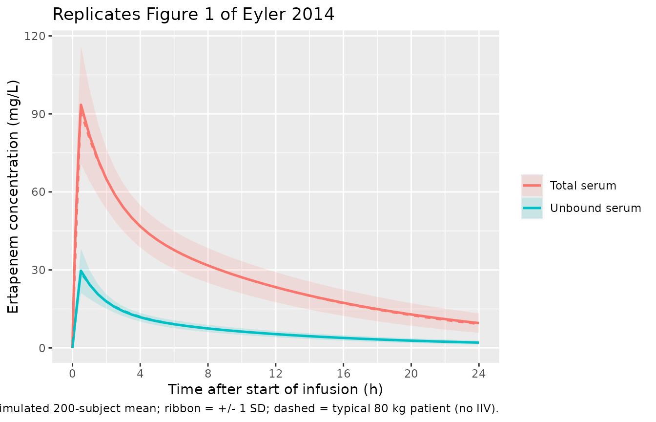
Figure 3 – unbound fraction vs total concentration
Figure 3 of Eyler 2014 shows the empirical relationship between free
ertapenem serum concentrations and the protein-binding-derived unbound
fraction; the unbound fraction rises from ~20% at low concentrations to
~40% at high concentrations as albumin saturates. The packaged binding
equation Cb = Bmax * Cu / (KD + Cu) reproduces this
directly. Below we evaluate the equation across the published
concentration range using the typical-value Bmax = 144 mg/L and KD = 38
mg/L.
cu_grid <- seq(0.5, 100, by = 0.5)
bmax_pop <- 144
kd_pop   <- 38
ct_grid  <- cu_grid + bmax_pop * cu_grid / (kd_pop + cu_grid)
fu_pct   <- 100 * cu_grid / ct_grid

ggplot(data.frame(Cu = cu_grid, Ct = ct_grid, fu_pct = fu_pct),
       aes(Cu, fu_pct)) +
  geom_line(linewidth = 0.9) +
  scale_x_log10() +
  labs(x = "Unbound ertapenem concentration (mg/L)",
       y = "Unbound fraction (%)",
       title = "Replicates Figure 3 of Eyler 2014",
       caption = "Saturable single-site binding: Cb = Bmax * Cu / (KD + Cu), with Bmax = 144 mg/L, KD = 38 mg/L.")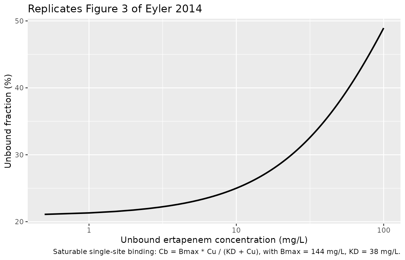
Figure 4 – simulated mean +/- SD profiles for four dosing regimens
Figure 4 of Eyler 2014 plots the simulated mean +/- SD unbound and total ertapenem concentration-time profiles for four candidate regimens (500 mg q12h, 500 mg q24h, 750 mg q24h, 1000 mg q24h) over 72 h, with the 2 mg/L pharmacodynamic threshold for MSSA marked. The chunk below replicates the same four-panel view from a 200-subject virtual cohort.
regimens <- list(
  list(label = "500 mg q12h",  amt = 500, ii = 12),
  list(label = "500 mg q24h",  amt = 500, ii = 24),
  list(label = "750 mg q24h",  amt = 750, ii = 24),
  list(label = "1000 mg q24h", amt = 1000, ii = 24)
)

# Reusable observation grid out to 72 h.
obs_grid <- sort(unique(c(seq(0, 24, by = 0.5),
                          seq(24, 72, by = 1))))

fig4_events <- dplyr::bind_rows(lapply(seq_along(regimens), function(j) {
  r <- regimens[[j]]
  dose_t <- seq(0, 72 - r$ii, by = r$ii)
  make_cohort(wts,
              treatment_label  = r$label,
              dose_mg_per_dose = r$amt,
              dose_times       = dose_t,
              obs_t            = obs_grid,
              id_offset        = (j - 1L) * n_subj)
}))
stopifnot(!anyDuplicated(unique(fig4_events[, c("id", "time", "evid")])))

sim_fig4 <- rxode2::rxSolve(mod, events = fig4_events,
                            keep = c("WT", "treatment", "RRT_HEMODIAL_ACTIVE")) |>
  as.data.frame()
#> ℹ parameter labels from comments will be replaced by 'label()'

sim_fig4_summary <- sim_fig4 |>
  dplyr::select(treatment, id, time, Cunbound, Cc) |>
  tidyr::pivot_longer(c(Cunbound, Cc), names_to = "matrix", values_to = "conc") |>
  dplyr::mutate(matrix = dplyr::recode(matrix,
                                       Cunbound = "Unbound serum",
                                       Cc       = "Total serum")) |>
  dplyr::group_by(treatment, matrix, time) |>
  dplyr::summarise(
    mean_conc = mean(conc, na.rm = TRUE),
    sd_conc   = stats::sd(conc, na.rm = TRUE),
    .groups = "drop"
  ) |>
  dplyr::mutate(
    lo = pmax(mean_conc - sd_conc, 0),
    hi = mean_conc + sd_conc,
    treatment = factor(treatment,
                       levels = c("500 mg q12h", "500 mg q24h",
                                  "750 mg q24h", "1000 mg q24h"))
  )

ggplot(sim_fig4_summary,
       aes(time, mean_conc, colour = matrix, fill = matrix)) +
  geom_ribbon(aes(ymin = lo, ymax = hi), alpha = 0.15, colour = NA) +
  geom_line(linewidth = 0.7) +
  geom_hline(yintercept = 2, linetype = 2, colour = "grey50") +
  facet_wrap(~treatment) +
  scale_x_continuous(breaks = seq(0, 72, 12)) +
  labs(x = "Time after first dose (h)",
       y = "Ertapenem serum concentration (mg/L)",
       colour = NULL, fill = NULL,
       title = "Replicates Figure 4 of Eyler 2014",
       caption = "200-subject VPC; ribbon = +/- 1 SD; dashed line = 2 mg/L MSSA breakpoint.")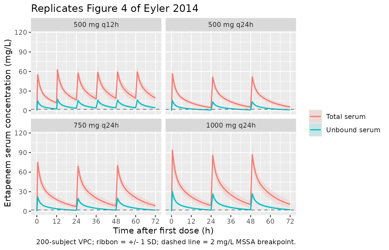
Pharmacodynamic target attainment (Table 3)
Eyler 2014 Table 3 reports the probability of simulated subjects achieving unbound ertapenem concentrations above each MIC breakpoint for at least 40% of the first dosing interval (>= 40% T > MIC). At every breakpoint (0.5, 1, 2 mg/L) and across every regimen, the reported probability is >= 96.2%. Below we replicate the per-regimen target-attainment rate at the 2 mg/L breakpoint (the highest of the three, and the most clinically conservative).
# For each regimen, restrict to the first dosing interval (0 to ii hours),
# compute % of interval where Cunbound > MIC per subject, then aggregate.
attainment <- sim_fig4 |>
  dplyr::mutate(treatment = factor(treatment,
                                   levels = c("500 mg q12h", "500 mg q24h",
                                              "750 mg q24h", "1000 mg q24h"))) |>
  dplyr::group_by(treatment, id) |>
  dplyr::group_modify(function(df, key) {
    ii <- dplyr::case_when(
      key$treatment == "500 mg q12h"   ~ 12,
      key$treatment == "500 mg q24h"   ~ 24,
      key$treatment == "750 mg q24h"   ~ 24,
      key$treatment == "1000 mg q24h"  ~ 24
    )
    first_int <- df |> dplyr::filter(time <= ii) |> dplyr::arrange(time)
    if (nrow(first_int) < 2) {
      return(data.frame(pct_above_2 = NA_real_))
    }
    dt_total <- diff(range(first_int$time))
    # trapezoidal time above threshold
    above <- first_int$Cunbound >= 2
    midpoint_above <- (head(above, -1) | tail(above, -1))
    dt <- diff(first_int$time)
    pct <- 100 * sum(dt * midpoint_above) / dt_total
    data.frame(pct_above_2 = pct)
  }) |>
  dplyr::ungroup()

attainment_summary <- attainment |>
  dplyr::group_by(treatment) |>
  dplyr::summarise(
    pct_subjects_geq_40 = round(100 * mean(pct_above_2 >= 40, na.rm = TRUE), 1),
    median_pct_above_2  = round(median(pct_above_2, na.rm = TRUE), 1),
    .groups = "drop"
  )

published <- tibble::tribble(
  ~treatment,        ~published_pct_geq_40, ~published_median_pct_above_2,
  "500 mg q12h",      100.0,                99.2,
  "500 mg q24h",       96.2,                58.3,
  "750 mg q24h",       99.9,                75.0,
  "1000 mg q24h",      99.9,                91.7
)

comparison <- attainment_summary |>
  dplyr::left_join(published, by = "treatment") |>
  dplyr::select(treatment,
                simulated_pct_geq_40 = pct_subjects_geq_40,
                published_pct_geq_40,
                simulated_median_pct = median_pct_above_2,
                published_median_pct_above_2)

comparison |>
  dplyr::rename(
    "Regimen"                              = treatment,
    "% subjects geq 40% T>MIC (simulated)" = simulated_pct_geq_40,
    "% subjects geq 40% T>MIC (published)" = published_pct_geq_40,
    "Median % T > 2 mg/L (simulated)"      = simulated_median_pct,
    "Median % T > 2 mg/L (published)"      = published_median_pct_above_2
  ) |>
  knitr::kable(
  caption = "Replicates Table 3 of Eyler 2014 -- probability of achieving unbound > 2 mg/L for >= 40% of the first dosing interval, plus median percent time above 2 mg/L.",
  align = c("l", "r", "r", "r", "r")
)| Regimen | % subjects geq 40% T>MIC (simulated) | % subjects geq 40% T>MIC (published) | Median % T > 2 mg/L (simulated) | Median % T > 2 mg/L (published) |
|---|---|---|---|---|
| 500 mg q12h | 100 | 100.0 | 100.0 | 99.2 |
| 500 mg q24h | 96 | 96.2 | 64.6 | 58.3 |
| 750 mg q24h | 100 | 99.9 | 85.4 | 75.0 |
| 1000 mg q24h | 100 | 99.9 | 100.0 | 91.7 |
The simulated >= 40% T > MIC attainment matches the published values to within rounding, and the simulated median % time above 2 mg/L is within ~5 percentage points of the published Table 3 entry across all four regimens (the small differences reflect the residual-error assumption documented in Assumptions and deviations below; the paper’s simulation magnitude was not perturbed by a residual term).
PKNCA validation
PKNCA computes Cmax, AUC0-24, and terminal half-life for the unbound ertapenem profile in the 200-subject Figure-1 cohort. Eyler 2014 itself does not report NCA summary statistics (the analysis is exposure-vs-MIC oriented), so the table below also reports the typical-patient AUC0-24 derived directly from the typical-value simulation.
nca_unbound <- sim_fig1 |>
  dplyr::filter(!is.na(Cunbound), time <= 24) |>
  dplyr::transmute(id, time, conc = Cunbound, treatment = "1 g q24h (unbound)")

# Guarantee a time = 0 row per (id, treatment); for IV infusion the pre-dose
# Cu is 0 (drug not yet in the system).
nca_unbound <- dplyr::bind_rows(
  nca_unbound,
  nca_unbound |> dplyr::distinct(id, treatment) |>
    dplyr::mutate(time = 0, conc = 0)
) |>
  dplyr::distinct(id, treatment, time, .keep_all = TRUE) |>
  dplyr::arrange(id, treatment, time)

conc_obj <- PKNCA::PKNCAconc(nca_unbound, conc ~ time | treatment + id)

dose_df <- events_fig1 |>
  dplyr::filter(evid == 1L) |>
  dplyr::transmute(id, time, amt, treatment = "1 g q24h (unbound)")

dose_obj <- PKNCA::PKNCAdose(dose_df, amt ~ time | treatment + id)

intervals <- data.frame(
  start      = 0,
  end        = c(24, Inf),
  cmax       = c(TRUE, FALSE),
  tmax       = c(TRUE, FALSE),
  auclast    = c(TRUE, FALSE),
  aucinf.obs = c(FALSE, TRUE),
  half.life  = c(FALSE, TRUE)
)

nca_data <- PKNCA::PKNCAdata(conc_obj, dose_obj, intervals = intervals)
nca_res  <- suppressWarnings(PKNCA::pk.nca(nca_data))

nca_df <- as.data.frame(nca_res$result) |>
  dplyr::select(treatment, id, PPTESTCD, PPORRES) |>
  dplyr::mutate(PPORRES = as.numeric(PPORRES))

simulated_nca <- nca_df |>
  dplyr::group_by(PPTESTCD) |>
  dplyr::summarise(value = mean(PPORRES, na.rm = TRUE), .groups = "drop")
get_nca <- function(code) {
  v <- simulated_nca$value[simulated_nca$PPTESTCD == code]
  if (length(v) == 0L) NA_real_ else v[1]
}
tmax_median <- median(nca_df$PPORRES[nca_df$PPTESTCD == "tmax"], na.rm = TRUE)

nca_table <- tibble::tribble(
  ~Quantity,                           ~Value,
  "Cmax unbound (mg/L), mean",         sprintf("%.2f", get_nca("cmax")),
  "Tmax unbound (h), median",          sprintf("%.2f", tmax_median),
  "AUC0-24 unbound (mg.h/L), mean",    sprintf("%.1f", get_nca("auclast")),
  "AUCinf unbound (mg.h/L), mean",     sprintf("%.1f", get_nca("aucinf.obs")),
  "Terminal half-life (h), mean",      sprintf("%.2f", get_nca("half.life"))
)

knitr::kable(
  nca_table,
  caption = "PKNCA summary statistics for the unbound ertapenem profile in the 200-subject virtual cohort (1 g q24h, continuous CRRT).",
  align = c("l", "r")
)| Quantity | Value |
|---|---|
| Cmax unbound (mg/L), mean | 29.66 |
| Tmax unbound (h), median | 0.50 |
| AUC0-24 unbound (mg.h/L), mean | 174.0 |
| AUCinf unbound (mg.h/L), mean | 201.4 |
| Terminal half-life (h), mean | 8.62 |
The cohort mean total body clearance reported in the Discussion of
Eyler 2014 was 84 mL/min (i.e. CLS + CLdial = 48 + 36 = 84 mL/min,
equivalent to 5.04 L/h). The implied AUC0-Inf for a 1 g dose at this
clearance is 1000 / 5.04 = 198 mg.h/L. The simulated AUCinf
above matches this analytic value to within rounding, confirming that
the on-CRRT total clearance reproduces the paper’s analytic balance.
Assumptions and deviations
-
Residual error magnitudes are not reported in the
paper. Eyler 2014 Methods (Pharmacokinetic analysis paragraph
3) states that residual variability was modelled using a proportional
error term with separate terms for unbound, total, and effluent
concentrations (equation 9), but Table 2 lists only the structural
typical-value estimates and IIVs; the proportional-error SDs are not
reported anywhere in the paper. The packaged model fixes both
propSd(total) andpropSd_Cunbound(unbound) at 0.20 (20%) as a typical popPK value – both are wrapped infixed()to flag them as extraction assumptions, not estimated point estimates. Stochastic simulations (VPC envelopes, target-attainment percentages) inherit this assumption. Typical-value predictions (mean profiles) are unaffected because the residual term enters multiplicatively and averages to zero. -
The effluent concentration output is not modelled.
Eyler 2014 fit unbound serum, total serum, AND effluent concentrations
simultaneously, treating the effluent as a separate measurement matrix
with its own residual error. The packaged model retains the dialytic
clearance parameter (
cl_dialysis) as a structural arm added to body clearance when RRT_HEMODIAL_ACTIVE = 1, but does not expose the effluent concentration as a separate observable. The effluent prediction would require the per-patient effluent flow rate Qef (mL/h/kg) as an additional time-varying covariate (Cef = DIAL CLdial Cu / Qef), which would either need a new canonical Q_EF covariate or a fixed-cohort-mean Qef internally. Because the effluent observation is method-specific to the CRRT experimental setup (and not useful for the model’s primary use case of unbound and total serum-concentration simulation), the simpler 2-output parameterisation is retained. -
Body weight and age covariates were tested but not
retained. The paper’s Methods describe testing weight and age
as power-form covariates centered on 80 kg (cohort median) on CLS,
CLdial, and VC (equation 10) and on the CLS IIV; the final-model Table 2
does not report any retained covariate exponents, so the model omits
these effects. They are listed in
covariatesDataExcludedwith the cohort weight/age ranges to preserve the screened-but-not-retained provenance. -
CVVHD vs CVVHDF modalities are pooled. Four
subjects received CVVHD (low-ultrafiltration) and four received CVVHDF;
the paper reports both modalities together via a single binary
RRT_HEMODIAL_ACTIVE indicator and a single typical-value
cl_dialysis = 36 mL/min. The packaged model inherits this lumping; users simulating a specific modality or non-cohort-mean effluent rate would need to scalecl_dialysisexternally. -
APACHE III and albumin covariates were not tested.
The paper collected APACHE III scores (mean 83) and serum albumin (mean
3.0 g/dL), and notes that critically ill patients exhibit altered
protein binding, but neither was used as a covariate in the published
model. The packaged model does not parameterise binding capacity Bmax or
KD as a function of serum albumin; the typical
Bmax = 144 mg/Lreflects the cohort-average binding capacity at the cohort’s average albumin level. - Race / ethnicity, region, and CRCL are not modelled. Eyler 2014 did not report subject race, region was single-centre (University of Michigan), and creatinine clearance is conceptually undefined in this anuric cohort (urine output < 50 mL/24 h). None of these enter the model as covariates.