Meropenem (Gijsen 2022)
Source:vignettes/articles/Gijsen_2022_meropenem.Rmd
Gijsen_2022_meropenem.RmdModel and source
#> ℹ parameter labels from comments will be replaced by 'label()'Citation: Gijsen M, Elkayal O, Annaert P, Van Daele R, Meersseman P, Debaveye Y, Wauters J, Dreesen E, Spriet I (2022). Meropenem Target Attainment and Population Pharmacokinetics in Critically Ill Septic Patients with Preserved or Increased Renal Function. Infection and Drug Resistance 15:53-62. doi:10.2147/IDR.S343264. Final parameter estimates from the NONMEM control stream in Supplementary File S2, cross-checked against Table 2.
Description: Two-compartment population PK model with linear elimination for intermittently infused meropenem (30-minute infusions) in critically ill adults with severe sepsis or septic shock and preserved or increased renal function (Gijsen 2022; 58 patients, 345 plasma concentrations over 70 dosing intervals, eGFR CKD-EPI >= 70 mL/min/1.73 m^2, no renal replacement therapy). Clearance (13.7 L/h at the reference) scales as a power function of Cockcroft-Gault creatinine clearance normalised to 111.7 mL/min (exponent 0.637); no other covariate was retained. Correlated interindividual variability on clearance and central volume, independent variability on peripheral volume, and combined proportional plus additive residual error.
Article: https://doi.org/10.2147/IDR.S343264
Gijsen and colleagues ran a prospective, rich-sampling population PK study of meropenem in critically ill septic adults whose renal function was preserved or increased, the group most at risk of underexposure to beta-lactams. A two-compartment model with linear elimination described the data, and Cockcroft-Gault creatinine clearance was the only covariate retained, as a power function on clearance. The paper also reported how often the unbound trough stayed above 2 mg/L and 8 mg/L (100% fT>MIC and 100% fT>4xMIC for an MIC of 2 mg/L). This vignette checks the packaged encoding against closed-form results, then simulates the study’s two main regimens and compares trough exposure and target attainment with Table 1.
Population
Fifty-eight adults (40 male, 69%) in the intensive care unit of University Hospitals Leuven, Belgium, with severe sepsis (45%) or septic shock (55%), contributed 345 plasma samples over 70 dosing intervals between October 2013 and October 2017. Median age was 63 years (IQR 55-68) and median weight 70 kg (IQR 60-79). APACHE II and SOFA scores on admission were 20 [16; 25] and 9 [7; 10]. Patients on renal replacement therapy or ECMO, and those with a CKD-EPI eGFR below 70 mL/min/1.73 m^2 on the sampling day, were excluded. Measured 24-hour urinary creatinine clearance was 84 [64; 119] and 109 [75; 136] mL/min/1.73 m^2 on early and late sampling days, and augmented renal clearance was present on 24.2% of dosing intervals.
Meropenem was given as 30-minute intermittent infusions: 1000 mg q8h on 64% of sampling days, 2000 mg q8h on most of the rest, and 500 mg q8h on two sampling days. Samples were drawn predose, at 30 (end of infusion), 120 and 240 minutes, and 15 minutes before the next dose (Gijsen 2022 Methods and Table 1).
The same information is available programmatically via the model’s
population metadata
(readModelDb("Gijsen_2022_meropenem")()$population).
Source trace
The final model is fully specified by the NONMEM control stream in
Supplementary File S2, whose $THETA and $OMEGA
values reproduce Table 2 to its printed precision (so they are final
estimates, not initial values). The per-parameter origin is also
recorded as an in-file comment next to each ini() entry in
inst/modeldb/specificDrugs/Gijsen_2022_meropenem.R.
| Equation / parameter | Value | Source location |
|---|---|---|
lcl (typical CL at CRCL = 111.7 mL/min) |
13.7 L/h | File S2 THETA(1); Table 2 CL row (RSE 7.4%) |
lvc (central volume) |
25.5 L | File S2 THETA(2); Table 2 Vc row (RSE 8.5%) |
lq (intercompartmental clearance) |
8.13 L/h | File S2 THETA(3); Table 2 Q = 8.1 L/h (RSE 32.6%) |
lvp (peripheral volume) |
12.4 L | File S2 THETA(4); Table 2 Vp row (RSE 15.8%) |
e_crcl_cl |
0.637 | File S2 THETA(5); Table 2 ‘eCrCl CG on CL’ = 0.64 (see Errata for Equation 2) |
var(etalcl) |
0.288 | File S2 $OMEGA BLOCK(2); Table 2 57.8% CV |
cov(etalcl, etalvc) |
0.185 | File S2 $OMEGA BLOCK(2) off-diagonal (see Errata) |
var(etalvc) |
0.281 | File S2 $OMEGA BLOCK(2); Table 2 57% CV |
var(etalvp) |
0.441 | File S2 second $OMEGA; Table 2 74.4% CV |
propSd |
sqrt(0.147) = 0.383 | File S2 $SIGMA first record, EPS(1) proportional (see
Errata) |
addSd |
sqrt(0.0925) = 0.304 mg/L | File S2 $SIGMA second record, EPS(2) additive (see
Errata) |
CL = 13.7 * (CRCL/111.7)^0.637 * exp(eta_CL) |
n/a | File S2 $PK; Results Equation 2 (reference 111.7
mL/min); Methods Equation 1 |
Vc, Vp exponential IIV; no IIV on
Q
|
n/a | File S2 $PK
|
| two-compartment ODEs | n/a | File S2 $DES
|
Cc ~ add(addSd) + prop(propSd) |
n/a | File S2 $ERROR:
W = SQRT(SIGMA(1,1)*IPRED**2 + SIGMA(2,2))
|
Structural verification
These checks do not depend on a random draw, so tight bounds are correct.
Variance scale against Table 2
Table 2 reports each variability term as
CV% = sqrt(exp(omega^2) - 1) x 100 (its abbreviations
footnote). Applying that formula to the packaged variances must return
the printed CVs. The same formula applied to the additive residual
variance returns the 31.1% that Table 2 prints on its proportional row,
which is the evidence for the label swap described in the Errata.
om <- ui$omega
cv_pct <- function(v) 100 * sqrt(exp(v) - 1)
var_chk <- data.frame(
  term = c("IIV on CL", "IIV on Vc", "IIV on Vp", "additive residual variance"),
  packaged_variance = c(om["etalcl", "etalcl"], om["etalvc", "etalvc"],
                        om["etalvp", "etalvp"], 0.3041^2),
  table2_cv_pct = c(57.8, 57, 74.4, 31.1)
) |>
  dplyr::mutate(cv_pct_from_variance = cv_pct(packaged_variance))

knitr::kable(
  var_chk |>
    dplyr::rename("Term" = term,
                  "Packaged variance" = packaged_variance,
                  "Table 2 CV (%)" = table2_cv_pct,
                  "sqrt(exp(v) - 1) x 100" = cv_pct_from_variance),
  digits = c(0, 4, 1, 2),
  caption = "Packaged variances back-transformed with the Table 2 CV formula."
)| Term | Packaged variance | Table 2 CV (%) | sqrt(exp(v) - 1) x 100 |
|---|---|---|---|
| IIV on CL | 0.2880 | 57.8 | 57.77 |
| IIV on Vc | 0.2810 | 57.0 | 56.96 |
| IIV on Vp | 0.4410 | 74.4 | 74.45 |
| additive residual variance | 0.0925 | 31.1 | 31.13 |
# Table 2 prints one decimal (57 for Vc); rounding error is at most 0.05.
stopifnot(max(abs(var_chk$cv_pct_from_variance - var_chk$table2_cv_pct)) < 0.1)

cat(sprintf("correlation between etalcl and etalvc: %.3f\n",
            om["etalcl", "etalvc"] / sqrt(om["etalcl", "etalcl"] * om["etalvc", "etalvc"])))
#> correlation between etalcl and etalvc: 0.650
Covariate relation
The solved individual clearance must equal the File S2 covariate equation.
typ <- rxode2::zeroRe(ui)
crcl_grid <- c(50, 80, 111.7, 150, 250)
ev_cov <- do.call(rbind, lapply(seq_along(crcl_grid), function(i) {
  data.frame(id = i, time = c(0, 1), amt = c(1000, 0), rate = c(2000, 0),
             evid = c(1, 0), cmt = "central", CRCL = crcl_grid[i])
}))
cov_chk <- rxode2::rxSolve(typ, ev_cov, returnType = "data.frame") |>
  dplyr::group_by(id) |>
  dplyr::summarise(CRCL = CRCL[1], cl_solved = cl[1], .groups = "drop") |>
  dplyr::mutate(cl_equation = 13.7 * (CRCL / 111.7)^0.637,
                rel_err = abs(cl_solved / cl_equation - 1))
#> ℹ omega/sigma items treated as zero: 'etalcl', 'etalvc', 'etalvp'
#> Warning: multi-subject simulation without without 'omega'

knitr::kable(
  cov_chk |>
    dplyr::select(-id) |>
    dplyr::rename("CRCL (mL/min)" = CRCL,
                  "CL solved (L/h)" = cl_solved,
                  "CL = 13.7 x (CRCL/111.7)^0.637 (L/h)" = cl_equation,
                  "Relative error" = rel_err),
  digits = c(1, 3, 3, 12),
  caption = "Typical clearance across creatinine clearance."
)| CRCL (mL/min) | CL solved (L/h) | CL = 13.7 x (CRCL/111.7)^0.637 (L/h) | Relative error |
|---|---|---|---|
| 50.0 | 8.210 | 8.210 | 0 |
| 80.0 | 11.076 | 11.076 | 0 |
| 111.7 | 13.700 | 13.700 | 0 |
| 150.0 | 16.530 | 16.530 | 0 |
| 250.0 | 22.888 | 22.888 | 0 |
Closed-form steady state
For a linear two-compartment model given a zero-order infusion of
rate R over T every tau, the
steady-state concentration is a sum of two exponentials with an exact
closed form. The ODE solve and the closed form use the same individual
parameters, so the difference is integrator error only.
# One exponential phase with rate li and unit-impulse coefficient ai: the
# current infusion plus the geometric sum of all earlier ones.
css_phase <- function(t, li, ai, r, tinf, tau) {
  cur <- ifelse(t <= tinf,
                1 - exp(-li * t),
                (1 - exp(-li * tinf)) * exp(-li * (t - tinf)))
  past <- (1 - exp(-li * tinf)) * exp(-li * (t - tinf)) * exp(-li * tau) /
    (1 - exp(-li * tau))
  r * ai / li * (cur + past)
}

# Vectorised over rows: every argument may be a per-row vector.
css_2cmt <- function(t, cl, vc, q, vp, dose, tinf, tau) {
  k10 <- cl / vc; k12 <- q / vc; k21 <- q / vp
  s <- k10 + k12 + k21
  alpha <- (s + sqrt(s^2 - 4 * k10 * k21)) / 2
  beta <- (s - sqrt(s^2 - 4 * k10 * k21)) / 2
  a_alpha <- (alpha - k21) / (vc * (alpha - beta))
  a_beta <- (k21 - beta) / (vc * (alpha - beta))
  r <- dose / tinf
  css_phase(t, alpha, a_alpha, r, tinf, tau) + css_phase(t, beta, a_beta, r, tinf, tau)
}

set.seed(2022)
n_cf <- 20
cf_par <- data.frame(id = seq_len(n_cf), CRCL = exp(rnorm(n_cf, log(111.7), 0.4)))
obs_t <- c(seq(0, 0.5, by = 0.05), seq(0.75, 8, by = 0.25))
ev_cf <- do.call(rbind, lapply(seq_len(n_cf), function(i) {
  rbind(
    data.frame(id = i, time = 0, amt = 2000, rate = 4000, ii = 8, ss = 1,
               evid = 1, cmt = "central", CRCL = cf_par$CRCL[i]),
    data.frame(id = i, time = obs_t, amt = 0, rate = 0, ii = 0, ss = 0,
               evid = 0, cmt = "central", CRCL = cf_par$CRCL[i])
  )
}))

rxode2::rxSetSeed(2022)
sim_cf <- rxode2::rxSolve(ui, ev_cf, returnType = "data.frame",
                          rtol = 1e-10, atol = 1e-12, ssRtol = 1e-10, ssAtol = 1e-12,
                          maxsteps = 1e6)
cf <- sim_cf |>
  dplyr::mutate(Cc_closed = css_2cmt(time, cl, vc, q, vp, dose = 2000, tinf = 0.5, tau = 8),
                rel_err = abs(Cc / Cc_closed - 1))

cat(sprintf("max relative error vs closed form: %.3g\n", max(cf$rel_err)))
#> max relative error vs closed form: 1.71e-10
# Tight tolerances on the solve; realised error is orders of magnitude below
# this bound, while a wrong micro-constant or infusion rate moves it by percent.
stopifnot(max(cf$rel_err) < 1e-5)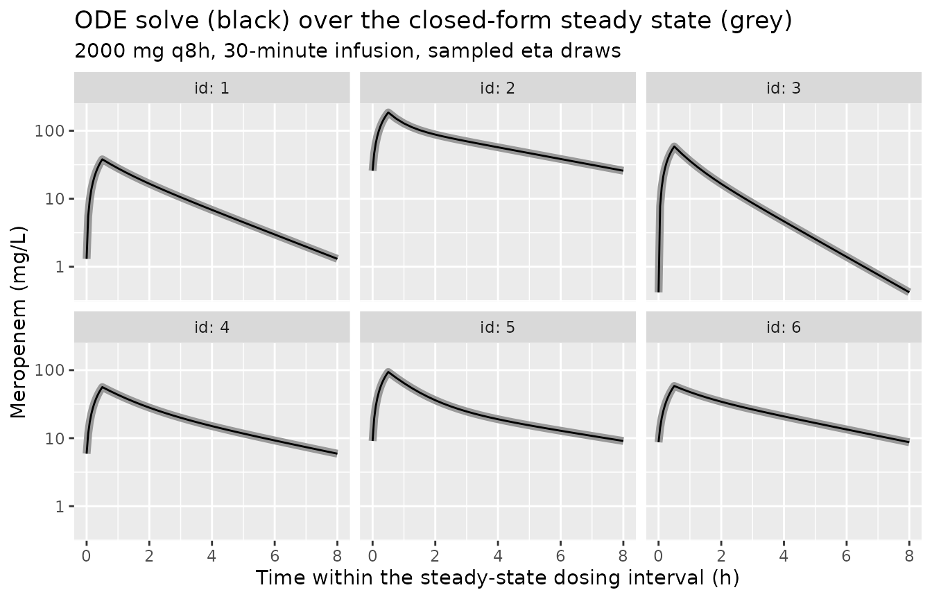
Virtual cohort
The observed data are not public. The paper does not tabulate the Cockcroft-Gault creatinine clearance of the cohort; it reports only the model reference of 111.7 mL/min. The cohort below draws CRCL log-normally around that reference, with a spread matching the interquartile range of measured urinary creatinine clearance (overall median 88, IQR 69-128 mL/min/1.73 m^2, a log IQR of 0.62 and so a log SD of about 0.46). Values outside 50-300 mL/min are redrawn, consistent with the eGFR >= 70 inclusion criterion. Two arms of 200 patients each receive the study’s main regimens, 1000 mg and 2000 mg q8h as 30-minute infusions, simulated at steady state.
# set.seed() fixes the covariate draw. rxSetSeed() fixes rxode2's eta and
# residual draws within one rxode2 build and thread count only, so the
# assertions below are on medians and robust proportions, never on extremes.
set.seed(20220111)
n_arm <- 200
draw_crcl <- function(n) {
  x <- exp(rnorm(n, log(111.7), 0.46))
  bad <- x < 50 | x > 300
  while (any(bad)) {
    x[bad] <- exp(rnorm(sum(bad), log(111.7), 0.46))
    bad <- x < 50 | x > 300
  }
  x
}

regimens <- data.frame(treatment = c("1000 mg q8h", "2000 mg q8h"), dose = c(1000, 2000))
cohort <- do.call(rbind, lapply(seq_len(nrow(regimens)), function(j) {
  data.frame(id = (j - 1) * n_arm + seq_len(n_arm),
             treatment = regimens$treatment[j],
             dose = regimens$dose[j],
             CRCL = draw_crcl(n_arm))
}))

obs_grid <- sort(unique(c(seq(0, 0.5, by = 0.05), seq(0.6, 8, by = 0.1), 7.75)))
events <- do.call(rbind, lapply(seq_len(nrow(cohort)), function(i) {
  p <- cohort[i, ]
  rbind(
    data.frame(id = p$id, time = 0, amt = p$dose, rate = p$dose / 0.5, ii = 8,
               ss = 1, evid = 1, cmt = "central", CRCL = p$CRCL,
               treatment = p$treatment),
    data.frame(id = p$id, time = obs_grid, amt = 0, rate = 0, ii = 0, ss = 0,
               evid = 0, cmt = "central", CRCL = p$CRCL,
               treatment = p$treatment)
  )
}))

summary(cohort$CRCL)
#>    Min. 1st Qu.  Median    Mean 3rd Qu.    Max.
#>   50.21   86.03  117.63  126.96  156.33  294.05
Simulation
rxode2::rxSetSeed(20220111)
sim <- rxode2::rxSolve(ui, events, returnType = "data.frame", maxsteps = 1e6,
                       keep = "treatment")
stopifnot(!anyNA(sim$Cc))
Steady-state profiles over one dosing interval
Figure 1 of the paper plots observed unbound concentrations over one dosing interval against the 2 and 8 mg/L targets. The figure below shows the simulated median and 5th-95th percentile band (with residual error) at the paper’s sampling design for each regimen.
prof <- sim |>
  dplyr::group_by(treatment, time) |>
  dplyr::summarise(p05 = quantile(sim, 0.05), p50 = median(sim),
                   p95 = quantile(sim, 0.95), .groups = "drop")

ggplot(prof, aes(time, p50)) +
  geom_ribbon(aes(ymin = pmax(p05, 0.05), ymax = p95), alpha = 0.25) +
  geom_line() +
  geom_hline(yintercept = c(2, 8), linetype = "dashed") +
  facet_wrap(~treatment) +
  scale_y_log10() +
  labs(x = "Time after start of infusion (h)",
       y = "Meropenem (mg/L)",
       title = "Simulated steady-state concentrations (median and 90% interval)",
       caption = "Compare with Figure 1 of Gijsen 2022; dashed lines are the 2 and 8 mg/L targets.")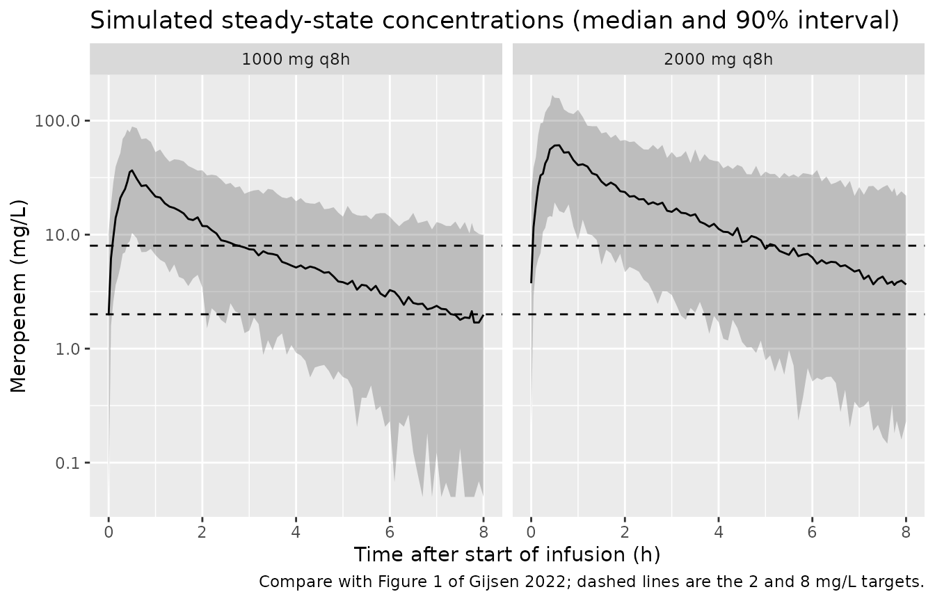
Trough concentrations and target attainment
Table 1 reports the unbound pre-dose concentration against the 2 and 8 mg/L targets. Total concentrations were treated as unbound in the paper (2% protein binding), so the simulated total concentration at 7.75 h (the sample drawn 15 minutes before the next dose) is compared directly. Residual error is included because the observed troughs carry it. The pooled simulated values weight the arms 45:23, the approximate split of the 68 non-500 mg sampling days (64% of 70 received 1000 mg; two received 500 mg).
trough <- sim |>
  dplyr::filter(abs(time - 7.75) < 1e-8) |>
  dplyr::select(id, treatment, CRCL, trough = sim)

by_arm <- trough |>
  dplyr::group_by(treatment) |>
  dplyr::summarise(median_trough = median(trough),
                   q25 = quantile(trough, 0.25), q75 = quantile(trough, 0.75),
                   ta2 = mean(trough >= 2), ta8 = mean(trough >= 8), .groups = "drop")

w <- c(`1000 mg q8h` = 45, `2000 mg q8h` = 23)
pooled_w <- w[trough$treatment] / as.numeric(table(trough$treatment)[trough$treatment])
wq <- function(x, wt, p) {
  o <- order(x); cw <- cumsum(wt[o]) / sum(wt)
  x[o][which(cw >= p)[1]]
}
pooled <- data.frame(
  treatment = "Pooled (45:23)",
  median_trough = wq(trough$trough, pooled_w, 0.5),
  q25 = wq(trough$trough, pooled_w, 0.25),
  q75 = wq(trough$trough, pooled_w, 0.75),
  ta2 = sum(pooled_w * (trough$trough >= 2)) / sum(pooled_w),
  ta8 = sum(pooled_w * (trough$trough >= 8)) / sum(pooled_w)
)
observed <- data.frame(treatment = "Observed (Table 1 / Results)", median_trough = 1.83,
                       q25 = 0.73, q75 = 4.85, ta2 = 32 / 70, ta8 = 8 / 70)

knitr::kable(
  dplyr::bind_rows(by_arm, pooled, observed) |>
    dplyr::mutate(ta2 = 100 * ta2, ta8 = 100 * ta8) |>
    dplyr::rename("Group" = treatment,
                  "Median trough (mg/L)" = median_trough,
                  "25th pct" = q25, "75th pct" = q75,
                  "Trough >= 2 mg/L (%)" = ta2,
                  "Trough >= 8 mg/L (%)" = ta8),
  digits = c(0, 2, 2, 2, 0, 0),
  caption = "Simulated steady-state troughs vs the observed values of Gijsen 2022."
)| Group | Median trough (mg/L) | 25th pct | 75th pct | Trough >= 2 mg/L (%) | Trough >= 8 mg/L (%) |
|---|---|---|---|---|---|
| 1000 mg q8h | 2.13 | 0.76 | 4.64 | 52 | 8 |
| 2000 mg q8h | 3.62 | 1.43 | 9.11 | 66 | 28 |
| Pooled (45:23) | 2.31 | 0.87 | 6.10 | 57 | 15 |
| Observed (Table 1 / Results) | 1.83 | 0.73 | 4.85 | 46 | 11 |
# Centre-of-distribution checks (robust to which subjects land in the tails).
# A 10-fold error in clearance, volume or dose shifts the median trough far
# outside a factor-of-two window around the observed 1.83 mg/L.
stopifnot(pooled$median_trough > 1.83 / 2, pooled$median_trough < 1.83 * 2)
The simulated pooled median trough is 2.31 mg/L against the observed 1.83 mg/L, and the simulated proportions of troughs at or above 2 and 8 mg/L are 57% and 15% against the observed 46% and 11%. The virtual cohort’s creatinine clearance distribution is an assumption (see below), so agreement is expected at the level of the centre of the distribution, not exactly.
Renal function drives trough exposure. The typical-value trough across creatinine clearance shows why most patients with preserved or augmented renal function miss the 8 mg/L target on standard doses:
crcl_seq <- seq(50, 250, by = 5)
ev_typ <- do.call(rbind, lapply(seq_len(nrow(regimens)), function(j) {
  do.call(rbind, lapply(seq_along(crcl_seq), function(i) {
    id <- (j - 1) * length(crcl_seq) + i
    rbind(
      data.frame(id = id, time = 0, amt = regimens$dose[j], rate = regimens$dose[j] / 0.5,
                 ii = 8, ss = 1, evid = 1, cmt = "central", CRCL = crcl_seq[i],
                 treatment = regimens$treatment[j]),
      data.frame(id = id, time = 7.75, amt = 0, rate = 0, ii = 0, ss = 0, evid = 0,
                 cmt = "central", CRCL = crcl_seq[i], treatment = regimens$treatment[j])
    )
  }))
}))
typ_trough <- rxode2::rxSolve(typ, ev_typ, returnType = "data.frame",
                              keep = "treatment", maxsteps = 1e6) |>
  dplyr::filter(time == 7.75)
#> ℹ omega/sigma items treated as zero: 'etalcl', 'etalvc', 'etalvp'
#> Warning: multi-subject simulation without without 'omega'

# Typical trough falls monotonically as CRCL rises (the only covariate).
stopifnot(all(tapply(typ_trough$Cc, typ_trough$treatment, function(x) all(diff(x) < 0))))
# The model is linear, so at the same CRCL the 2000 mg trough is exactly twice
# the 1000 mg trough (same parameters on both sides; integrator error only).
dose_ratio <- typ_trough$Cc[typ_trough$treatment == "2000 mg q8h"] /
  typ_trough$Cc[typ_trough$treatment == "1000 mg q8h"]
stopifnot(max(abs(dose_ratio - 2)) < 1e-3)

ggplot(typ_trough, aes(CRCL, Cc, colour = treatment)) +
  geom_line(linewidth = 1) +
  geom_hline(yintercept = c(2, 8), linetype = "dashed") +
  labs(x = "Cockcroft-Gault creatinine clearance (mL/min)",
       y = "Typical steady-state trough (mg/L)", colour = NULL,
       title = "Typical trough at 7.75 h vs renal function")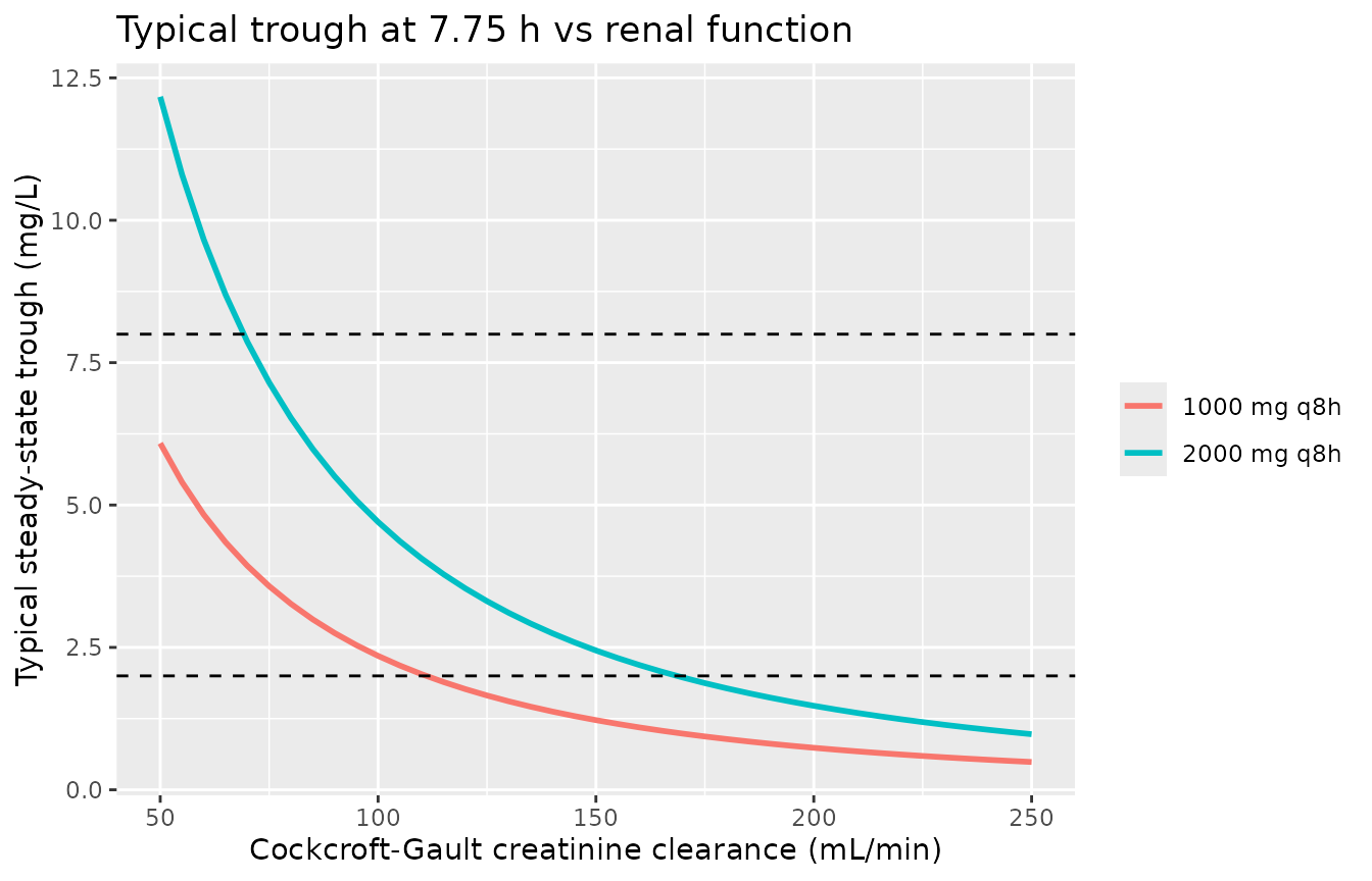
PKNCA validation
Non-compartmental analysis over the steady-state dosing interval (0-8
h) on the individual predictions. At steady state the interval AUC must
equal Dose / CL for every subject, which checks mass
balance independently of the closed form above. The paper reports no NCA
of its own.
conc <- sim |>
  dplyr::filter(!is.na(Cc)) |>
  dplyr::select(id, time, Cc, treatment)
dose_df <- events |>
  dplyr::filter(evid == 1) |>
  dplyr::select(id, time, amt, treatment)

o_conc <- PKNCA::PKNCAconc(conc, Cc ~ time | treatment + id)
o_dose <- PKNCA::PKNCAdose(dose_df, amt ~ time | treatment + id)
intervals <- data.frame(start = 0, end = 8, cmax = TRUE, tmax = TRUE, cmin = TRUE,
                        auclast = TRUE, cav = TRUE)
nca <- PKNCA::pk.nca(PKNCA::PKNCAdata(o_conc, o_dose, intervals = intervals))
nca_res <- as.data.frame(nca$result)

nca_summary <- nca_res |>
  dplyr::group_by(treatment, PPTESTCD) |>
  dplyr::summarise(median = median(PPORRES), .groups = "drop") |>
  tidyr::pivot_wider(names_from = PPTESTCD, values_from = median)

knitr::kable(
  nca_summary |>
    dplyr::select(treatment, cmax, tmax, cmin, auclast, cav) |>
    dplyr::rename("Regimen" = treatment, "Cmax (mg/L)" = cmax, "Tmax (h)" = tmax,
                  "Cmin (mg/L)" = cmin, "AUC0-8 (mg*h/L)" = auclast,
                  "Cavg (mg/L)" = cav),
  digits = 2,
  caption = "Median steady-state NCA parameters (simulated, individual predictions)."
)| Regimen | Cmax (mg/L) | Tmax (h) | Cmin (mg/L) | AUC0-8 (mg*h/L) | Cavg (mg/L) |
|---|---|---|---|---|---|
| 1000 mg q8h | 34.69 | 0.5 | 1.89 | 74.09 | 9.26 |
| 2000 mg q8h | 68.40 | 0.5 | 3.64 | 145.65 | 18.21 |
auc_chk <- nca_res |>
  dplyr::filter(PPTESTCD == "auclast") |>
  dplyr::left_join(sim |> dplyr::distinct(id, cl), by = "id") |>
  dplyr::left_join(cohort |> dplyr::select(id, dose), by = "id") |>
  dplyr::mutate(rel_err = PPORRES * cl / dose - 1)

cat(sprintf("AUC0-8 x CL / Dose - 1: median %.2g, 99th pct |err| %.2g\n",
            median(auc_chk$rel_err), quantile(abs(auc_chk$rel_err), 0.99)))
#> AUC0-8 x CL / Dose - 1: median 1.2e-05, 99th pct |err| 0.00018
# Trapezoidal error on a 0.05-0.1 h grid around a 30-minute infusion peak is
# well under 1%; a wrong clearance, dose or infusion handling moves this by
# tens of percent.
stopifnot(abs(median(auc_chk$rel_err)) < 0.01,
          quantile(abs(auc_chk$rel_err), 0.9) < 0.02)
Assumptions and deviations
- Covariate distribution. The paper does not tabulate Cockcroft-Gault creatinine clearance. The virtual cohort draws it log-normally around the model reference of 111.7 mL/min, with a spread borrowed from the measured 24-hour urinary creatinine clearance IQR and a 50-300 mL/min window. The trough and target-attainment comparison therefore tests the centre of the exposure distribution, not its tails.
- Regimen mix. The two 500 mg q8h sampling days are not simulated; the pooled summary weights 1000 mg and 2000 mg q8h 45:23.
- Target attainment definition. The paper required the unbound concentration to exceed the target throughout the interval, judged from the two pre-dose samples. The simulation uses the single steady-state trough at 7.75 h (the pre-dose sample of the next interval, which equals the pre-dose sample of the current interval at steady state), with residual error.
- Steady state. Patients were sampled on day 2 +/- 1 or 5 +/- 1 of therapy. With a typical half-life of a few hours, steady state is assumed.
-
Cockcroft-Gault body weight. The paper does not say
whether total, ideal or adjusted body weight entered the Cockcroft-Gault
equation. The
CRCLcolumn should be computed the same way as in the source, which is unknown; total body weight is the conventional default. - Reference CRCL. The paper does not state which statistic 111.7 mL/min is. It is used as the normalising constant exactly as in File S2.
Errata
-
Equation 2 exponent. The Results print Equation 2
as
CL_i = 13.7 L/h x (eCrClCG / 111.7 mL/min)^0.725. The control stream in File S2 (THETA(5) = 0.637), Table 2 (0.64) and the bootstrap median (0.64) all agree on 0.637, so 0.725 is treated as a typographical error and 0.637 is used. -
Residual error labels in Table 2 are swapped. File
S2 codes
Y = IPRED * (1 + EPS(1)) + EPS(2)with$SIGMAvalues 0.147 (commented ‘prop err’) and 0.0925 (commented ‘add err’). Table 2 instead reports an additive residual of ‘0.147 mg/L’ and a proportional residual of ‘31.1 %CV’. The 31.1% is exactlysqrt(exp(0.0925) - 1), the back-transformed additive variance, and 0.147 is the untransformed proportional variance. The model encodes the as-run control stream: proportional SDsqrt(0.147)= 0.383 and additive SDsqrt(0.0925)= 0.304 mg/L. The two readings give the same total residual SD at about 1 mg/L (near the troughs) and differ only at higher concentrations. -
Covariance printed as a correlation. Table 2 lists
‘Correlation between CL & Vc’ as 0.185. In File S2 0.185 is the
off-diagonal element of
$OMEGA BLOCK(2), which NONMEM reads as a covariance; the implied correlation is 0.65. The covariance is encoded. - Units of the additive residual. Table 2 gives the additive residual in mg/L while printing a variance; the encoded additive SD is in mg/L.