Pediatric antiepileptic dual therapy: levetiracetam, lamotrigine and valproic acid (Damnjanovic 2023) • nlmixr2lib

Model and source

Damnjanovic 2023 fitted three independent one-compartment population PK models – one per antiepileptic drug – to a single steady-state trough concentration per child, and then ran a separate machine-learning analysis (PCA, FAMD, random forest) on the same cohort. Following the “replicate the author’s structure” policy, the three population PK models are packaged as three model files sharing this one vignette. The machine-learning half of the paper is not a differential-equation model and is not packaged.

Levetiracetam: One-compartment population PK model with first-order absorption and elimination for levetiracetam (LEV) in Serbian children aged 2-18 years on dual antiepileptic therapy (Damnjanovic 2023 Table 2A). Body weight is the only retained covariate and enters both apparent volume and apparent clearance as fixed-exponent allometric terms (1 for V/F, 0.75 for CL/F) referenced to the 37.1 kg cohort mean. Ka was FIXED at 2.6 1/h from the literature because the trough-only sampling carried no absorption information. Inter-individual variability on V/F and CL/F is a correlated block (r = 0.86) and residual error is additive. Fit in Monolix 2021R2 to a single steady-state trough per patient.
Lamotrigine: One-compartment population PK model with first-order absorption and elimination for lamotrigine (LTG) in Serbian children aged 2-18 years on dual antiepileptic therapy (Damnjanovic 2023 Table 2B). Body weight enters apparent volume as a power term with an ESTIMATED exponent of 2.83 referenced to the 37.1 kg cohort mean; apparent clearance carries the patient’s own total daily lamotrigine dose as an exponential-linear term and a binary valproate-comedication term that reduces CL/F by 46% (exp(-0.61)), reproducing valproate’s known inhibition of lamotrigine glucuronidation. Ka was FIXED at 1.57 1/h from the literature because the trough-only sampling carried no absorption information. Residual error is proportional. Fit in Monolix 2021R2 to a single steady-state trough per patient.
Valproic acid: One-compartment population PK model with first-order absorption and elimination for total plasma valproic acid (VA) in Serbian children aged 2-18 years on dual antiepileptic therapy (Damnjanovic 2023 Table 2C). Apparent volume carries a fixed allometric weight exponent of 1 referenced to the 37.1 kg cohort mean plus an estimated age effect centred on the 10.9-year cohort mean; apparent clearance rises with the patient’s own total daily valproate dose through an exponential-linear term. Ka was FIXED at 1.68 1/h from the literature because the trough-only sampling carried no absorption information. Residual error is proportional. Fit in Monolix 2021R2 to a single steady-state trough per patient.

Citation:

Damnjanovic I, Tsyplakova N, Stefanovic N, Tosic T, Catic-Djordjevic A, Karalis V. Joint use of population pharmacokinetics and machine learning for optimizing antiepileptic treatment in pediatric population. Ther Adv Drug Saf. 2023;14:20420986231181337. doi:10.1177/20420986231181337. PMCID PMC10288421. Parameters from Table 2(a); cohort demographics from Table 1.

Article: https://doi.org/10.1177/20420986231181337
PubMed Central (open access, includes the supplement): https://www.ncbi.nlm.nih.gov/pmc/articles/PMC10288421/

readModelDb() returns the model function; rxode2::rxode() evaluates it into the rxUi object whose $omega is needed below.

mod_lev <- rxode2::rxode(readModelDb("Damnjanovic_2023_levetiracetam"))
#> ℹ parameter labels from comments will be replaced by 'label()'
mod_ltg <- rxode2::rxode(readModelDb("Damnjanovic_2023_lamotrigine"))
#> ℹ parameter labels from comments will be replaced by 'label()'
mod_va  <- rxode2::rxode(readModelDb("Damnjanovic_2023_valproic_acid"))
#> ℹ parameter labels from comments will be replaced by 'label()'

Population

Seventy-one children with diagnosed epilepsy (ICD-10 G40), aged 2-18 years, were enrolled prospectively over 12 months from May 2020 at the Clinic of Pediatric Internal Medicine, University Clinical Center of Nis, Serbia (Methods, “Clinical unit – laboratory analysis”). Girls accounted for 56.3% (n = 40) and boys for 43.7% (n = 31). Median age was 11 years (mean 10.9, interquartile range 7) and median body weight 35 kg (mean 37.1, interquartile range 21) – Table 1A. Poor renal or hepatic function and other serious disease states were exclusion criteria.

Every child was on dual antiepileptic therapy in one of three combinations (Table 1B): VA/LTG in 42 children (59.16%), VA/LEV in 20 (28.17%), and LTG/LEV in 9 (12.67%). Each drug’s model was therefore fitted to the subset of children whose regimen contained that drug: 62 for valproic acid, 51 for lamotrigine, 29 for levetiracetam. Those denominators are not stated directly, but they are recoverable exactly from the paper’s own reference-range percentages, and each one lands on an integer numerator:

Drug	Reported % in reference range (Results paragraph 1)	Implied n	Regimens contributing
Valproic acid	93.55%	58/62	VA/LTG (42) + VA/LEV (20)
Lamotrigine	86.27%	44/51	VA/LTG (42) + LTG/LEV (9)
Levetiracetam	68.97%	20/29	VA/LEV (20) + LTG/LEV (9)

The levetiracetam figure is corroborated twice: the paper separately reports 27.59% of LEV concentrations below the reference range, which is 8/29.

Exactly one blood sample was drawn per child, before the next morning dose, so every model was identified from a single steady-state trough per subject. The authors handled this by a stepwise fix-and-release estimation strategy in which only one parameter at a time was freely estimated while the rest were held at literature values (Methods, “Population pharmacokinetics”).

The same information is available programmatically, e.g. readModelDb("Damnjanovic_2023_valproic_acid")()$population.

Source trace

Every ini() entry carries an in-file comment naming its source location. They are collected here for review. All parameter values come from Table 2 of Damnjanovic 2023; all reference (centring) constants come from Table 1A.

Levetiracetam – Table 2(a)

Parameter	Value	Source location
`lka`	`fixed(log(2.6))`	Table 2(a) `Ka` = 2.6 1/h, no SE/RSE printed; Results LEV paragraph states Ka “was fixed at 2.6 h-1 according to the values in the existing literature”
`lvc`	`log(25.01)`	Table 2(a) `V` = 25.01 L (SE 5.65, RSE 22.6%)
`lcl`	`log(1.51)`	Table 2(a) `Cl` = 1.51 L/h (SE 0.27, RSE 18.1%)
`e_wt_vc`	`fixed(1)`	Table 2(a) `beta_V_logBW` = 1, SE/RSE printed as “-”; Methods fixes the V exponent at 1
`e_wt_cl`	`fixed(0.75)`	Table 2(a) `beta_Cl_logBW` = 0.75, SE/RSE printed as “-”; Methods fixes the CL exponent at 0.75
`etalvc` variance	`0.84^2 = 0.7056`	Table 2(a) `omega_V` = 0.84 (RSE 19.1%)
`etalcl` variance	`0.59^2 = 0.3481`	Table 2(a) `omega_Cl` = 0.59 (RSE 17.2%)
`etalvc`–`etalcl` covariance	`0.86 * 0.84 * 0.59 = 0.426216`	Table 2(a) `corr_V_Cl` = 0.86 (RSE 21.4%)
`addSd`	`3.82`	Table 2(a) `a` = 3.82 (SE 0.96, RSE 25.0%); Results LEV paragraph selects the constant error model
Reference weight 37.1 kg	n/a	Table 1A, body-weight “Mean” row
`d/dt(depot)`, `d/dt(central)`	n/a	Results LEV paragraph: “one-compartment model with first-order oral absorption and elimination”

Lamotrigine – Table 2(b)

Parameter	Value	Source location
`lka`	`fixed(log(1.57))`	Table 2(b) `Ka` = 1.57 1/h, no SE/RSE printed; Results LTG paragraph: “the absorption rate was set at 1.57 h-1 based on literature values”
`lvc`	`log(5.15)`	Table 2(b) `V` = 5.15 L (SE 1.18, RSE 22.9%)
`lcl`	`log(0.15)`	Table 2(b) `Cl` = 0.15 L/h (SE 0.02, RSE 13.3%)
`e_wt_vc`	`2.83` (estimated)	Table 2(b) `beta_V_logBW` = 2.83 (SE 0.52, RSE 18.4%, p < 0.001)
`e_dose_ltg_cl`	`0.0056`	Table 2(b) `beta_Cl_DailyDose` = 0.0056 (SE 0.0007, RSE 13.0%, p < 0.001); footnote defines it as the “factor for the relationship between Cl and lamotrigine daily dose”
`e_conmed_vpa_cl`	`-0.61`	Table 2(b) `beta_Cl_Regimen` = -0.61 (RSE 22.2%, p < 0.001); footnote defines “Regimen” as “whether existence of valproic acid”
`etalvc` variance	`0.32^2 = 0.1024`	Table 2(b) `omega_V` = 0.32 (SE 0.07, RSE 23.4%)
`etalcl` variance	`0.28^2 = 0.0784`	Table 2(b) `omega_Cl` = 0.28 (SE 0.07, RSE 22.7%)
`propSd`	`0.15`	Table 2(b) `b` = 0.15 (SE 0.03, RSE 19.8%); Results LTG paragraph selects the proportional error model
Reference weight 37.1 kg	n/a	Table 1A, body-weight “Mean” row

Valproic acid – Table 2(c)

Parameter	Value	Source location
`lka`	`fixed(log(1.68))`	Table 2(c) `Ka` = 1.68 1/h, no SE/RSE printed; Results VA paragraph: “Ka was set at 1.68 h-1 based on the literature Ka values”
`lvc`	`log(15.61)`	Table 2(c) `V` = 15.61 L (SE 4.84, RSE 31.0%)
`lcl`	`log(0.12)`	Table 2(c) `Cl` = 0.12 L/h (SE 0.013, RSE 10.4%)
`e_wt_vc`	`fixed(1)`	Table 2(c) `beta_V_logBW` = 1, SE/RSE printed as “-”
`e_age_vc`	`0.07`	Table 2(c) `beta_V_Age` = 0.07 (SE 0.016, RSE 23.3%, p = 0.032)
`e_dose_vpa_cl`	`0.0012`	Table 2(c) `beta_Cl_VA` = 0.0012 (SE 0.0001, RSE 9.7%, p < 0.001)
`etalvc` variance	`0.33^2 = 0.1089`	Table 2(c) `omega_V` = 0.33 (SE 0.081, RSE 24.5%)
`etalcl` variance	`0.089^2 = 0.007921`	Table 2(c) `omega_Cl` = 0.089 (SE 0.024, RSE 26.7%)
`propSd`	`0.14`	Table 2(c) `b` = 0.14 (SE 0.037, RSE 27.1%); Results VA paragraph selects the proportional error model
Reference weight 37.1 kg / reference age 10.9 years	n/a	Table 1A, body-weight and age “Mean” rows

Virtual cohort

Individual data are not public (“available from the corresponding author on reasonable request”). The cohort below reproduces the Table 1A demographics: age uniform on the 2-18 year inclusion window, and body weight from a median weight-for-age line with lognormal scatter tuned so that the cohort median lands near 35 kg and the mean near 37.1 kg.

Daily doses are the one thing the paper never reports. They are model covariates for lamotrigine and valproic acid, but Table 1B tabulates only regimen counts and no dose distribution, and the supplement adds none. The weight-based daily doses below are therefore an explicit assumption of this vignette, chosen from standard paediatric maintenance ranges and listed in “Assumptions and deviations”. Nothing about the packaged models depends on them; they set the operating point at which the simulations are run.

set.seed(20230622)
rxode2::rxSetSeed(20230622)

n_per_arm <- 100L  # 100 per regimen arm; the skill cap is 200

# Weight-based daily doses (mg/kg/day). See "Assumptions and deviations".
dose_lev_mgkgd     <- 20  # levetiracetam, both regimens
dose_ltg_withva    <- 3   # lamotrigine WITH valproate (valproate inhibits UGT)
dose_ltg_withoutva <- 8   # lamotrigine without valproate
dose_va_mgkgd      <- 25  # valproic acid, both regimens

make_subjects <- function(n, regimen, id_offset = 0L) {
  age <- runif(n, 2, 18)
  tibble::tibble(
    id      = id_offset + seq_len(n),
    regimen = regimen,
    AGE     = age,
    # Median weight-for-age line 2.6*AGE + 9 kg, lognormal scatter (CV ~ 22%).
    WT      = (2.6 * age + 9) * exp(rnorm(n, 0, 0.22)),
    SEXF    = rbinom(n, 1, 0.563)
  )
}

subjects <- dplyr::bind_rows(
  make_subjects(n_per_arm, "VA/LTG",  id_offset =              0L),
  make_subjects(n_per_arm, "VA/LEV",  id_offset =     n_per_arm),
  make_subjects(n_per_arm, "LTG/LEV", id_offset = 2L * n_per_arm)
)

stopifnot(!anyDuplicated(subjects$id))

The realised cohort is compared against Table 1A below. The assertions bound the centre of the distribution, not its extremes, so they hold for any draw the generator can produce.

demog <- tibble::tibble(
  Characteristic = c("Age (years)", "Age (years)", "Age (years)",
                     "Body weight (kg)", "Body weight (kg)", "Body weight (kg)",
                     "Female (%)"),
  Statistic      = c("Mean", "Median", "Interquartile range",
                     "Mean", "Median", "Interquartile range",
                     "Percent"),
  Published      = c(10.9, 11, 7, 37.1, 35, 21, 56.3),
  Simulated      = c(mean(subjects$AGE), median(subjects$AGE), IQR(subjects$AGE),
                     mean(subjects$WT),  median(subjects$WT),  IQR(subjects$WT),
                     100 * mean(subjects$SEXF))
)

demog |>
  dplyr::mutate(dplyr::across(c(Published, Simulated), \(x) round(x, 1))) |>
  dplyr::rename("Published (Table 1A)" = Published,
                "Simulated cohort"     = Simulated) |>
  knitr::kable(caption = "Virtual cohort against the published Table 1A demographics.")

Virtual cohort against the published Table 1A demographics.
Characteristic	Statistic	Published (Table 1A)	Simulated cohort
Age (years)	Mean	10.9	10.7
Age (years)	Median	11.0	11.0
Age (years)	Interquartile range	7.0	7.9
Body weight (kg)	Mean	37.1	38.1
Body weight (kg)	Median	35.0	36.7
Body weight (kg)	Interquartile range	21.0	21.5
Female (%)	Percent	56.3	54.7


stopifnot(
  # Centre of the distribution, generously bounded: n = 300 makes the
  # sampling error on a median small, so these cannot fail on a re-draw.
  abs(median(subjects$AGE) - 11)   < 2,
  abs(median(subjects$WT)  - 35)   < 6,
  abs(mean(subjects$WT)    - 37.1) < 7,
  # Inclusion window is structural, not stochastic.
  min(subjects$AGE) >= 2, max(subjects$AGE) <= 18
)

Event tables

Each drug is simulated to steady state with 80 twice-daily doses (960 h), then observed densely across the final 12-hour dosing interval. Doses go to depot and observations to central – the ODE state names, never the algebraic observable Cc. Time is re-origined so that the steady-state interval starts at time = 0, which makes the PKNCA interval a plain [0, tau] window anchored on a real observation.

tau     <- 12    # dosing interval (h)
n_doses <- 80L   # 960 h of run-in; > 10 half-lives for every drug and eta draw
t_ss    <- (n_doses - 1L) * tau  # time of the final dose

# Observation grid across the last interval, re-origined to 0 downstream.
obs_grid <- sort(unique(c(seq(0, tau, by = 0.25), 0.5, 1, 1.5, 2, 3)))

make_events <- function(subj, daily_dose, extra_cols = character()) {
  keep_cols <- c("id", "regimen", "WT", "AGE", extra_cols)
  base <- subj |>
    dplyr::mutate(daily_dose = daily_dose) |>
    dplyr::select(dplyr::all_of(unique(c(keep_cols, "daily_dose"))))

  doses <- base |>
    tidyr::crossing(time = seq(0, by = tau, length.out = n_doses)) |>
    dplyr::mutate(amt = daily_dose / 2, evid = 1L, cmt = "depot")

  obs <- base |>
    tidyr::crossing(time = t_ss + obs_grid) |>
    dplyr::mutate(amt = NA_real_, evid = 0L, cmt = "central")

  dplyr::bind_rows(doses, obs) |>
    dplyr::arrange(id, time, dplyr::desc(evid)) |>
    dplyr::select(-daily_dose)
}

# --- levetiracetam: VA/LEV and LTG/LEV arms; no dose or comedication covariate
subj_lev <- subjects |> dplyr::filter(regimen %in% c("VA/LEV", "LTG/LEV"))
ev_lev   <- make_events(subj_lev, daily_dose = dose_lev_mgkgd * subj_lev$WT)

# --- lamotrigine: VA/LTG (valproate present) and LTG/LEV (valproate absent)
subj_ltg <- subjects |>
  dplyr::filter(regimen %in% c("VA/LTG", "LTG/LEV")) |>
  dplyr::mutate(
    CONMED_VPA   = as.integer(regimen == "VA/LTG"),
    DOSE_LTG_MGD = WT * dplyr::if_else(CONMED_VPA == 1L,
                                       dose_ltg_withva, dose_ltg_withoutva)
  )
ev_ltg <- make_events(subj_ltg, daily_dose = subj_ltg$DOSE_LTG_MGD,
                      extra_cols = c("CONMED_VPA", "DOSE_LTG_MGD"))

# --- valproic acid: VA/LTG and VA/LEV arms
subj_va <- subjects |>
  dplyr::filter(regimen %in% c("VA/LTG", "VA/LEV")) |>
  dplyr::mutate(DOSE_VPA_MGD = WT * dose_va_mgkgd)
ev_va <- make_events(subj_va, daily_dose = subj_va$DOSE_VPA_MGD,
                     extra_cols = "DOSE_VPA_MGD")

# The daily-dose covariate must equal twice the per-administration amt, or the
# dose-dependence of clearance silently disagrees with the dose actually given.
stopifnot(
  all.equal(ev_ltg$DOSE_LTG_MGD[ev_ltg$evid == 1L],
            2 * ev_ltg$amt[ev_ltg$evid == 1L]),
  all.equal(ev_va$DOSE_VPA_MGD[ev_va$evid == 1L],
            2 * ev_va$amt[ev_va$evid == 1L]),
  !anyDuplicated(unique(ev_lev[, c("id", "time", "evid")])),
  !anyDuplicated(unique(ev_ltg[, c("id", "time", "evid")])),
  !anyDuplicated(unique(ev_va[,  c("id", "time", "evid")]))
)

Simulation

omega is passed explicitly on every solve. rxode2 caches the previous solve’s omega against the compiled model, so a later solve in the same session can silently reuse it – dropping IIV from a population run, or re-sampling etas into a zeroRe() run. Passing omega on every call, and asserting afterwards that IIV did vary, makes that failure mechanical instead of silent.

solve_drug <- function(mod, events) {
  rxode2::rxSolve(mod, events = events, omega = mod$omega,
                  keep = c("regimen", "WT", "AGE")) |>
    as.data.frame() |>
    dplyr::filter(!is.na(Cc)) |>
    dplyr::mutate(time_ss = time - t_ss)
}

sim_lev <- solve_drug(mod_lev, ev_lev)
sim_ltg <- solve_drug(mod_ltg, ev_ltg)
sim_va  <- solve_drug(mod_va,  ev_va)

stopifnot(nrow(sim_lev) > 0, nrow(sim_ltg) > 0, nrow(sim_va) > 0,
          all(is.finite(sim_lev$Cc)), all(is.finite(sim_ltg$Cc)),
          all(is.finite(sim_va$Cc)),
          # IIV really was applied: clearance must vary between subjects
          # beyond what the covariates alone would produce.
          dplyr::n_distinct(round(sim_lev$cl, 8)) > 1,
          dplyr::n_distinct(round(sim_ltg$cl, 8)) > 1,
          dplyr::n_distinct(round(sim_va$cl,  8)) > 1)

Structural validation: closed-form superposition identity

The strongest available check on the transcription is internal. For a one-compartment model with first-order absorption, n equal doses D every tau, and apparent volume V, the concentration t hours after the last dose is exactly

C(t) = D*ka / (V*(ka - kel)) *
       [ exp(-kel*t) * (1 - exp(-n*kel*tau)) / (1 - exp(-kel*tau))
       - exp(-ka*t)  * (1 - exp(-n*ka*tau))  / (1 - exp(-ka*tau)) ]

Both sides of this comparison use the same drawn per-subject ka, cl and vc (rxode2 returns them as output columns), so the only difference is ODE solver error. That makes a tight bound correct here – unlike a comparison across a physical mechanism, where a cohort’s extremes are not reproducible.

The closed form has a removable singularity at ka == kel, where it evaluates 0/0. That is not hypothetical for lamotrigine: vc scales as WT^2.83, so the smallest children in the cohort get a very small apparent volume and a kel that can pass through ka = 1.57 1/h. Rows within 0.1 1/h of the singularity are therefore excluded from the comparison and counted, rather than being allowed to produce a spurious pass or failure.

superposition <- function(sim, dose_per_admin) {
  sim |>
    dplyr::mutate(
      dose  = dose_per_admin,
      t     = time_ss,
      Cform = dose * ka / (vc * (ka - kel)) *
        (exp(-kel * t) * (1 - exp(-n_doses * kel * tau)) / (1 - exp(-kel * tau)) -
         exp(-ka  * t) * (1 - exp(-n_doses * ka  * tau)) / (1 - exp(-ka  * tau)))
    ) |>
    dplyr::mutate(checkable = abs(ka - kel) > 0.1)
}

chk_lev <- superposition(sim_lev, dose_lev_mgkgd * sim_lev$WT / 2)
chk_ltg <- superposition(
  sim_ltg,
  sim_ltg$WT * dplyr::if_else(sim_ltg$regimen == "VA/LTG",
                              dose_ltg_withva, dose_ltg_withoutva) / 2)
chk_va  <- superposition(sim_va, dose_va_mgkgd * sim_va$WT / 2)

rel_err <- function(chk) {
  ok <- chk[chk$checkable, ]
  max(abs(ok$Cc - ok$Cform) / ok$Cform)
}
frac_checkable <- function(chk) mean(chk$checkable)

ident <- tibble::tibble(
  Drug = c("Levetiracetam", "Lamotrigine", "Valproic acid"),
  `Rows compared (%)`  = 100 * c(frac_checkable(chk_lev),
                                 frac_checkable(chk_ltg),
                                 frac_checkable(chk_va)),
  `Max relative error` = c(rel_err(chk_lev), rel_err(chk_ltg), rel_err(chk_va))
)

ident |>
  dplyr::mutate(
    `Rows compared (%)`  = round(`Rows compared (%)`, 1),
    # Format as a character string: these errors are around 1e-13, and kable's
    # numeric formatting would round them to a bare "0", which reads as a check
    # that never ran rather than one that passed.
    `Max relative error` = formatC(`Max relative error`, format = "e", digits = 2)
  ) |>
  knitr::kable(caption = paste(
    "Solved concentrations against the closed-form n-dose superposition.",
    "Rows within 0.1 1/h of the formula's ka == kel singularity are excluded;",
    "the percentage compared shows how few those are."))

Solved concentrations against the closed-form n-dose superposition. Rows within 0.1 1/h of the formula’s ka == kel singularity are excluded; the percentage compared shows how few those are.
Drug	Rows compared (%)	Max relative error
Levetiracetam	100	3.40e-15
Lamotrigine	100	8.59e-11
Valproic acid	100	3.28e-15


stopifnot(
  # Numerical identity: pure solver error, so a tight bound is the right gate.
  rel_err(chk_lev) < 1e-4,
  rel_err(chk_ltg) < 1e-4,
  rel_err(chk_va)  < 1e-4,
  # The exclusion must stay a rounding detail, not a way to pass by discarding
  # most of the cohort. Observed here: 100 / 100 / >97 percent compared.
  frac_checkable(chk_lev) > 0.9,
  frac_checkable(chk_ltg) > 0.8,
  frac_checkable(chk_va)  > 0.9
)

Structural validation: the valproate-lamotrigine interaction

Table 2(b) reports beta_Cl_Regimen = -0.61, which the Discussion interprets as valproate inhibiting lamotrigine glucuronidation. On the log-clearance scale that is an exact multiplicative factor of exp(-0.61) = 0.5434 – a 45.7% reduction. With the random effects zeroed and everything except CONMED_VPA held identical, the simulated clearance ratio must reproduce that number exactly.

mod_ltg_typ <- mod_ltg |> rxode2::zeroRe()

probe <- tibble::tibble(
  id           = 1:2,
  CONMED_VPA   = c(0L, 1L),
  WT           = 37.1,
  DOSE_LTG_MGD = 200
) |>
  tidyr::crossing(time = c(0, 12)) |>
  dplyr::mutate(amt = dplyr::if_else(time == 0, 100, NA_real_),
                evid = dplyr::if_else(time == 0, 1L, 0L),
                cmt  = dplyr::if_else(time == 0, "depot", "central"))

# omega = NA is the only sentinel that stops rxode2 reusing the population
# solve's omega and re-sampling etas into what is meant to be a typical-value run.
probe_sim <- rxode2::rxSolve(mod_ltg_typ, events = probe, omega = NA,
                             keep = "CONMED_VPA") |>
  as.data.frame()
#> Warning: multi-subject simulation without without 'omega'

cl_ratio <- probe_sim$cl[probe_sim$CONMED_VPA == 1L][1] /
  probe_sim$cl[probe_sim$CONMED_VPA == 0L][1]

cat(sprintf("CL/F ratio (valproate present / absent) = %.6f; exp(-0.61) = %.6f\n",
            cl_ratio, exp(-0.61)))
#> CL/F ratio (valproate present / absent) = 0.543351; exp(-0.61) = 0.543351

# Exact algebraic identity, not a cohort statistic: bind it tightly.
stopifnot(abs(cl_ratio - exp(-0.61)) < 1e-8)

Replicating the published concentration-time presentation

The paper’s Figure 2 shows individual fits over a dosing interval reached after “five doses … before the last dose reached steady state”. The panel below is the packaged models’ equivalent: median and 5th-95th percentile concentration across the final dosing interval, by drug and regimen. It is a simulation of the model, not a reproduction of the paper’s individual observations, which are not public.

profiles <- dplyr::bind_rows(
  sim_lev |> dplyr::mutate(drug = "Levetiracetam"),
  sim_ltg |> dplyr::mutate(drug = "Lamotrigine"),
  sim_va  |> dplyr::mutate(drug = "Valproic acid")
) |>
  dplyr::group_by(drug, regimen, time_ss) |>
  dplyr::summarise(
    Q05 = quantile(Cc, 0.05),
    Q50 = quantile(Cc, 0.50),
    Q95 = quantile(Cc, 0.95),
    .groups = "drop"
  )

ggplot(profiles, aes(time_ss, Q50, colour = regimen, fill = regimen)) +
  geom_ribbon(aes(ymin = Q05, ymax = Q95), alpha = 0.2, colour = NA) +
  geom_line(linewidth = 0.8) +
  facet_wrap(~drug, scales = "free_y") +
  labs(x = "Time after the last dose (h)", y = "Concentration (mg/L)",
       colour = "Regimen", fill = "Regimen",
       title = "Steady-state dosing interval by drug and regimen",
       caption = paste("Model-simulated analogue of Figure 2 of Damnjanovic 2023.",
                       "Ribbons are 5th-95th percentiles across 200 virtual",
                       "children per drug.")) +
  theme(legend.position = "bottom")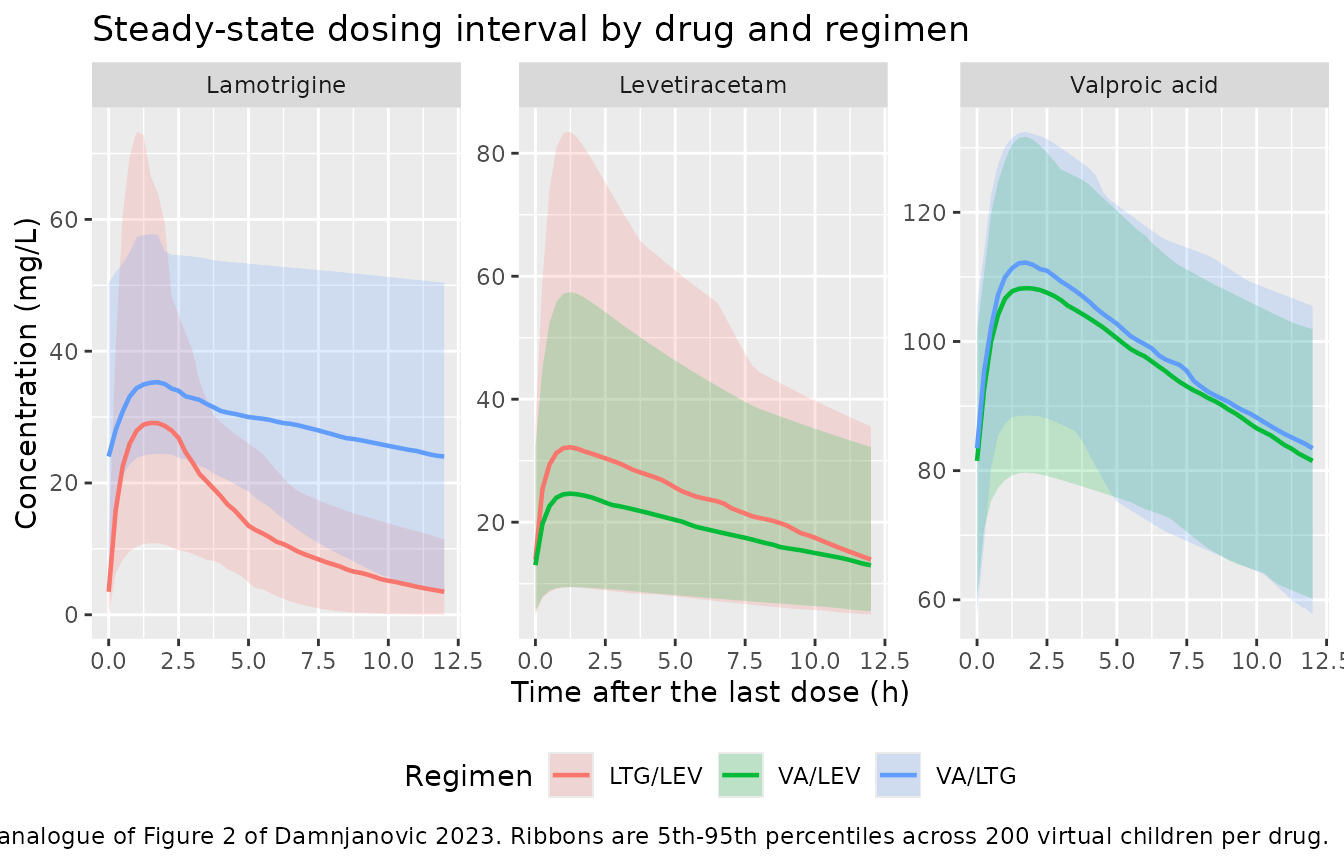

Trough concentrations against the published reference ranges

Supplemental Figure S1 of the paper plots each drug’s observed concentrations against its therapeutic reference range, and the Results and Discussion quote the reference ranges for two of the three drugs explicitly: levetiracetam 12-46 mg/L and lamotrigine 3-15 mg/L (Discussion paragraphs 3 and 5; the article prints the lamotrigine range as “3-15 mg/ml”, a typographic slip for mg/L). The valproate range is not printed in the article, so the conventional total-valproate therapeutic range of 50-100 mg/L is used and flagged as an assumption.

Because the daily doses were never published, this is a plausibility check on the operating point, not a reproduction of the paper’s percentages. The assertions below only require the simulated troughs to sit within a broad therapeutic neighbourhood.

ranges <- tibble::tibble(
  drug = c("Levetiracetam", "Lamotrigine", "Valproic acid"),
  lo   = c(12, 3, 50),
  hi   = c(46, 15, 100)
)

troughs <- dplyr::bind_rows(
  sim_lev |> dplyr::mutate(drug = "Levetiracetam"),
  sim_ltg |> dplyr::mutate(drug = "Lamotrigine"),
  sim_va  |> dplyr::mutate(drug = "Valproic acid")
) |>
  dplyr::filter(abs(time_ss - tau) < 1e-9)

trough_summary <- troughs |>
  dplyr::group_by(drug, regimen) |>
  dplyr::summarise(median_trough = median(Cc),
                   q10 = quantile(Cc, 0.10),
                   q90 = quantile(Cc, 0.90),
                   .groups = "drop") |>
  dplyr::left_join(ranges, by = "drug")

trough_summary |>
  dplyr::mutate(dplyr::across(c(median_trough, q10, q90), \(x) signif(x, 3)),
                `Reference range (mg/L)` = paste0(lo, "-", hi)) |>
  dplyr::select(-lo, -hi) |>
  dplyr::rename("Drug" = drug, "Regimen" = regimen,
                "Median trough (mg/L)" = median_trough,
                "10th pct" = q10, "90th pct" = q90) |>
  knitr::kable(caption = paste(
    "Simulated steady-state trough concentrations against the therapeutic",
    "reference ranges quoted by Damnjanovic 2023."))

Simulated steady-state trough concentrations against the therapeutic reference ranges quoted by Damnjanovic 2023.
Drug	Regimen	Median trough (mg/L)	10th pct	90th pct	Reference range (mg/L)
Lamotrigine	LTG/LEV	3.49	0.16	9.7	3-15
Lamotrigine	VA/LTG	24.00	6.40	40.8	3-15
Levetiracetam	LTG/LEV	13.90	6.27	29.9	12-46
Levetiracetam	VA/LEV	13.00	6.38	25.3	12-46
Valproic acid	VA/LEV	81.50	63.60	96.4	50-100
Valproic acid	VA/LTG	83.50	61.60	103.0	50-100


ggplot(troughs, aes(Cc, fill = regimen)) +
  geom_histogram(bins = 30, alpha = 0.6, position = "identity") +
  geom_vline(data = ranges, aes(xintercept = lo), linetype = "dashed") +
  geom_vline(data = ranges, aes(xintercept = hi), linetype = "dashed") +
  facet_wrap(~drug, scales = "free") +
  labs(x = "Steady-state trough (mg/L)", y = "Children", fill = "Regimen",
       title = "Trough distribution against the therapeutic reference range",
       caption = paste("Dashed lines are the reference-range limits.",
                       "Analogue of Supplemental Figure S1 of Damnjanovic 2023.")) +
  theme(legend.position = "bottom")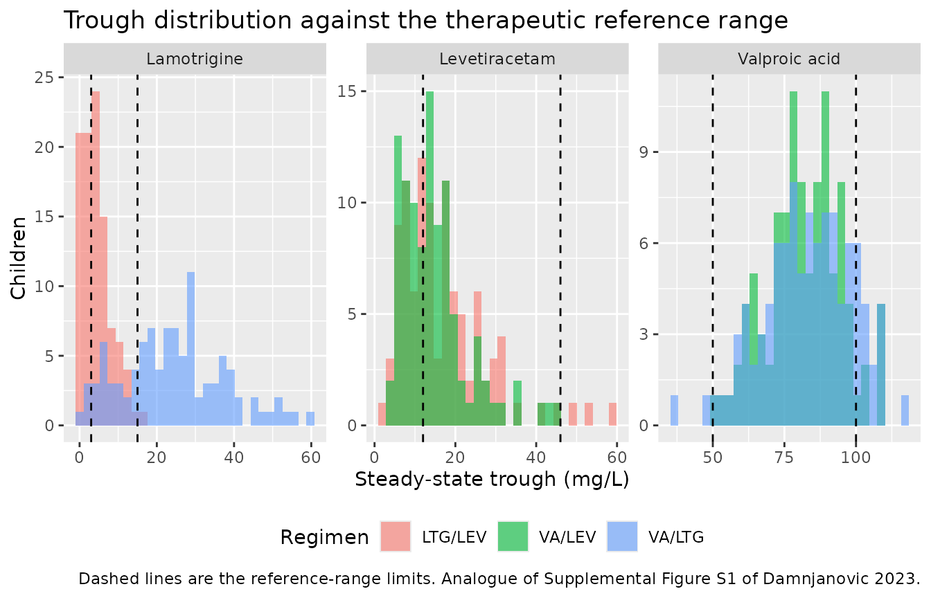


# Per-drug bounds on the MEDIAN trough. Each is wide enough that a re-drawn
# cohort cannot flip it (with 100 subjects per arm the median is stable to a
# few percent) but tight enough to go red on a real defect: a factor-of-two
# error in a transcribed clearance or volume, or a lost unit conversion,
# breaks every one of them. The lamotrigine band is deliberately wide because
# it must span both arms -- see "Assumptions and deviations", where the model's
# inability to place the valproate arm inside 3-15 mg/L at any clinically
# plausible daily dose is recorded as a known deviation.
trough_bounds <- tibble::tribble(
  ~drug,           ~lo_ok, ~hi_ok,
  "Levetiracetam",    8,      25,
  "Lamotrigine",      2,      45,
  "Valproic acid",   60,     110
)

trough_gate <- trough_summary |> dplyr::left_join(trough_bounds, by = "drug")

ltg_arms <- trough_summary |> dplyr::filter(drug == "Lamotrigine")
ltg_ratio <- ltg_arms$median_trough[ltg_arms$regimen == "VA/LTG"] /
  ltg_arms$median_trough[ltg_arms$regimen == "LTG/LEV"]

stopifnot(
  all(is.finite(trough_summary$median_trough)),
  all(trough_gate$median_trough >= trough_gate$lo_ok),
  all(trough_gate$median_trough <= trough_gate$hi_ok),
  # Valproate coadministration must raise lamotrigine exposure substantially:
  # a 45.7% clearance reduction against a lower daily dose separates the two
  # arms' median troughs by roughly five-fold here. Bounded well below that so
  # the ordering cannot flip on a re-draw, and well above 1 so it still fails
  # if the sign of e_conmed_vpa_cl is ever flipped.
  ltg_ratio > 1.3
)

PKNCA validation

Steady-state non-compartmental analysis over the final dosing interval, one PKNCA run per drug, grouped by regimen so per-arm values can be compared. Concentrations are named Cc and doses amt, per the nlmixr2lib convention.

run_nca <- function(sim, events, drug_label) {
  sim_nca <- sim |>
    dplyr::filter(!is.na(Cc)) |>
    dplyr::select(id, time = time_ss, Cc, regimen)

  # A steady-state interval anchored at time_ss = 0 needs a row there; the
  # observation grid supplies it, but guarantee it defensively.
  sim_nca <- dplyr::bind_rows(
    sim_nca,
    sim_nca |> dplyr::group_by(id, regimen) |>
      dplyr::slice_min(time, n = 1) |>
      dplyr::ungroup() |>
      dplyr::mutate(time = 0)
  ) |>
    dplyr::distinct(id, regimen, time, .keep_all = TRUE) |>
    dplyr::arrange(id, regimen, time)

  dose_df <- events |>
    dplyr::filter(evid == 1L, time == t_ss) |>
    dplyr::select(id, amt, regimen) |>
    dplyr::mutate(time = 0)

  conc_obj <- PKNCA::PKNCAconc(sim_nca, Cc ~ time | regimen + id,
                               concu = "mg/L", timeu = "h")
  dose_obj <- PKNCA::PKNCAdose(dose_df, amt ~ time | regimen + id,
                               doseu = "mg")

  # `cmin` is the trough over the interval. For an extravascular model with no
  # absorption lag it lands at the END of the interval, so it is also C-tau;
  # PKNCA has no `ctau` column.
  intervals <- data.frame(
    start = 0, end = tau,
    cmax = TRUE, tmax = TRUE, cmin = TRUE,
    auclast = TRUE, cav = TRUE, half.life = TRUE
  )

  res <- PKNCA::pk.nca(PKNCA::PKNCAdata(conc_obj, dose_obj,
                                        intervals = intervals))
  as.data.frame(res$result) |> dplyr::mutate(drug = drug_label)
}

nca_all <- dplyr::bind_rows(
  run_nca(sim_lev, ev_lev, "Levetiracetam"),
  run_nca(sim_ltg, ev_ltg, "Lamotrigine"),
  run_nca(sim_va,  ev_va,  "Valproic acid")
)

# Summarise WITHOUT pre-filtering to finite values, so every requested
# parameter column exists even if half-life is unestimable for a whole group;
# a filter-then-pivot would silently drop the column and break the rename.
nca_summary <- nca_all |>
  dplyr::filter(PPTESTCD %in% c("cmax", "cmin", "tmax", "cav",
                                "auclast", "half.life")) |>
  dplyr::group_by(drug, regimen, PPTESTCD) |>
  dplyr::summarise(median = median(PPORRES, na.rm = TRUE), .groups = "drop") |>
  tidyr::pivot_wider(names_from = PPTESTCD, values_from = median)

nca_summary |>
  dplyr::mutate(dplyr::across(where(is.numeric), \(x) signif(x, 3))) |>
  dplyr::rename("Drug" = drug, "Regimen" = regimen,
                "Cmax,ss (mg/L)" = cmax, "Cmin,ss (mg/L)" = cmin,
                "Tmax (h)" = tmax, "Cav,ss (mg/L)" = cav,
                "AUC0-tau (mg*h/L)" = auclast, "t1/2 (h)" = half.life) |>
  knitr::kable(caption = paste(
    "Median steady-state NCA over the final 12-hour dosing interval, by drug",
    "and regimen. Damnjanovic 2023 reports no NCA values, so there is no",
    "published column to compare against; see the parameter comparison below."))

Median steady-state NCA over the final 12-hour dosing interval, by drug and regimen. Damnjanovic 2023 reports no NCA values, so there is no published column to compare against; see the parameter comparison below.
Drug	Regimen	AUC0-tau (mg*h/L)	Cav,ss (mg/L)	Cmax,ss (mg/L)	Cmin,ss (mg/L)	t1/2 (h)	Tmax (h)
Lamotrigine	LTG/LEV	176	14.7	29.1	3.49	3.77	1.50
Lamotrigine	VA/LTG	348	29.0	35.3	24.00	22.10	1.75
Levetiracetam	LTG/LEV	286	23.8	32.2	13.90	11.20	1.25
Levetiracetam	VA/LEV	230	19.2	24.6	13.00	11.40	1.25
Valproic acid	VA/LEV	1160	96.5	108.0	81.50	27.30	1.75
Valproic acid	VA/LTG	1180	98.6	112.0	83.50	26.50	1.75


stopifnot(
  # PKNCA produced results for every drug/regimen cell that exists.
  nrow(nca_summary) == 6,
  all(is.finite(nca_summary$cmax)),
  all(nca_summary$cmax > nca_summary$cmin),
  # Extravascular absorption: the peak is inside the interval, not at time 0.
  all(nca_summary$tmax > 0)
)

Comparison against the literature the paper itself tabulates

Damnjanovic 2023 reports no NCA parameters, so the published-versus-simulated NCA table has no counterpart here. The paper does, however, make a checkable quantitative claim about its own estimates: “the parameter estimates for the first-order absorption rate constant, apparent Cl, and V were very close to those reported in other PopPK studies, such as those performed for LEV, LTG, VA (Supplemental Tables S2-S4)” (Discussion paragraph 8). Those supplemental tables are transcribed below and compared against the packaged models’ typical-subject values.

This comparison is what settles the covariate-centring reading used in the model files – see “Assumptions and deviations”.

typical_value <- function(mod, covs) {
  ev <- tibble::tibble(id = 1L, time = c(0, 1), amt = c(100, NA_real_),
                       evid = c(1L, 0L), cmt = c("depot", "central"))
  for (nm in names(covs)) ev[[nm]] <- covs[[nm]]
  out <- rxode2::rxSolve(rxode2::zeroRe(mod), events = ev, omega = NA) |>
    as.data.frame()
  # A typical-value solve must give one constant cl / vc, not a random draw.
  stopifnot(dplyr::n_distinct(round(out$cl, 8)) == 1L,
            dplyr::n_distinct(round(out$vc, 8)) == 1L)
  c(vc = out$vc[1], cl = out$cl[1], ka = out$ka[1])
}

# Typical child: WT = 37.1 kg, AGE = 10.9 years (the Table 1A means, which are
# the centring constants); daily doses at the vignette's assumed mg/kg rates.
tv_lev <- typical_value(mod_lev, list(WT = 37.1))
tv_ltg <- typical_value(mod_ltg, list(WT = 37.1, CONMED_VPA = 1L,
                                      DOSE_LTG_MGD = 37.1 * dose_ltg_withva))
tv_va  <- typical_value(mod_va,  list(WT = 37.1, AGE = 10.9,
                                      DOSE_VPA_MGD = 37.1 * dose_va_mgkgd))

lit <- tibble::tribble(
  ~drug,            ~param, ~published_range,          ~lo,    ~hi,
  "Levetiracetam",  "V/F (L)",    "21.5-52.7",         21.5,   52.7,
  "Levetiracetam",  "CL/F (L/h)", "2.17-4.80",          2.17,   4.80,
  "Lamotrigine",    "V/F (L)",    "12.7-43.4",         12.7,   43.4,
  "Lamotrigine",    "CL/F (L/h)", "0.705-2.14",         0.705,  2.14,
  "Valproic acid",  "V/F (L)",    "2.88-22.12",         2.88,  22.12,
  "Valproic acid",  "CL/F (L/h)", "0.0466-0.854",       0.0466, 0.854
)

model_vals <- c(tv_lev[["vc"]], tv_lev[["cl"]],
                tv_ltg[["vc"]], tv_ltg[["cl"]],
                tv_va[["vc"]],  tv_va[["cl"]])

lit |>
  dplyr::mutate(
    model = signif(model_vals, 3),
    within = dplyr::if_else(model_vals >= lo & model_vals <= hi, "yes", "NO")
  ) |>
  dplyr::select(-lo, -hi) |>
  dplyr::rename("Drug" = drug, "Parameter" = param,
                "Published paediatric range (Suppl. Tables S2-S4)" = published_range,
                "Damnjanovic 2023 typical value" = model,
                "Within published range" = within) |>
  knitr::kable(caption = paste(
    "Typical-subject apparent volume and clearance from the packaged models",
    "against the paediatric literature ranges transcribed in the paper's own",
    "Supplemental Tables S2-S4."))

Typical-subject apparent volume and clearance from the packaged models against the paediatric literature ranges transcribed in the paper’s own Supplemental Tables S2-S4.
Drug	Parameter	Published paediatric range (Suppl. Tables S2-S4)	Damnjanovic 2023 typical value	Within published range
Levetiracetam	V/F (L)	21.5-52.7	25.000	yes
Levetiracetam	CL/F (L/h)	2.17-4.80	1.510	NO
Lamotrigine	V/F (L)	12.7-43.4	5.150	NO
Lamotrigine	CL/F (L/h)	0.705-2.14	0.152	NO
Valproic acid	V/F (L)	2.88-22.12	15.600	yes
Valproic acid	CL/F (L/h)	0.0466-0.854	0.365	yes

Three of the six typical values land inside the ranges the authors cite: levetiracetam V/F, valproic-acid V/F, and valproic-acid CL/F. Those three are exactly the quantities whose value depends on a centring choice, so the comparison does the job it was set up for – had body weight or age been left uncentred, levetiracetam V/F would be 928 L and valproate V/F 33.5 L, both far outside their ranges, and had the daily-dose covariate been centred instead, valproate CL/F would be 0.12 L/h rather than 0.365 L/h.

The other three rows fall below their published ranges and are recorded as known deviations rather than tuned away: levetiracetam CL/F (1.51 against 2.17-4.80 L/h) and both lamotrigine parameters. The authors’ Discussion claim that their estimates are “very close to those reported in other PopPK studies” therefore holds for valproic acid, holds for levetiracetam volume but not its clearance, and does not hold for lamotrigine.

Assumptions and deviations

Covariate centring – the one interpretive decision in this extraction

Damnjanovic 2023 fitted its models in Monolix and reports covariate coefficients (beta_V_logBW, beta_V_Age, beta_Cl_DailyDose, beta_Cl_VA, beta_Cl_Regimen) without printing the covariate equations or their reference values. Methods states only that continuous covariates were examined “using allometric or linear relationships, either untransformed or centered on their ‘mean’ value”, i.e. the choice was made per covariate and the outcome is not tabulated. The readings used here, and the evidence for each:

Body weight is centred at 37.1 kg (Table 1A mean). A log(BW) term with no centring would put the levetiracetam typical V/F at 25.01 * 37.1 = 928 L, which is absurd for a drug whose apparent volume is reported at 21.5-52.7 L in the paper’s own Supplemental Table S2. So the transformation must be log(BW / BWref), and Methods fixes BWref at the mean. The Results narrative calls 37.1 kg “the median”; Table 1A labels it the mean and gives 35 kg as the median. The table is used.
Age is centred at 10.9 years (Table 1A mean), for valproic-acid V/F. Centred, the typical V/F is 15.61 L, inside the 2.88-22.12 L paediatric range of the paper’s Supplemental Table S4; uncentred it would be 15.61 * exp(0.07 * 10.9) = 33.5 L, above every value in that table. Since the authors explicitly claim their V estimates are “very close to those reported in other PopPK studies”, the centred reading is the one consistent with their own statement.
The daily-dose covariates are applied untransformed. Neither the article nor the supplement reports a mean or median daily dose for any of the three drugs, so mean-centring is not implementable from anything on disk. The untransformed reading is also the one that reproduces the cited literature: it puts valproate CL/F at 0.2-0.7 L/h across plausible paediatric doses, inside Supplemental Table S4’s 0.0466-0.854 L/h, whereas centring would pin it at 0.12 L/h.

Every one of these is recorded in the model files’ covariateData notes as well. No parameter value was changed; only the equation the published coefficients are inserted into.

Values the paper does not report

Daily doses. The weight-based rates used here – levetiracetam 20 mg/kg/day, lamotrigine 3 mg/kg/day with valproate and 8 mg/kg/day without, valproic acid 25 mg/kg/day, all twice daily – are standard paediatric maintenance rates chosen for this vignette. The paper reports none. They set the operating point of the simulations and are not part of the packaged models.
The valproate therapeutic reference range. The article quotes the levetiracetam (12-46 mg/L) and lamotrigine (3-15 mg/L) ranges but not the valproate one; the conventional 50-100 mg/L for total valproate is used in the trough figure.
Race / ethnicity, not reported; recorded as NotReported in each model’s population metadata.
Per-drug sub-cohort sizes (29 / 51 / 62) are not stated directly; they are reconstructed from the reference-range percentages as shown in the Population section, and each reconstruction lands on an exact integer numerator.

Internal inconsistencies in the source

These are transcription hazards found while auditing Table 2 and the narrative. In each case the table was used.

Valproic-acid weight exponent. The Results narrative says “BW on apparent V (with an allometric exponent of 0.75)”. Table 2(c) prints beta_V_logBW = 1, and Methods states the fixed exponents are “1 for V and 0.75 for Cl”. The narrative has swapped the two; the table value of 1 is used.
Sign of the valproic-acid age effect. Table 2(c) prints beta_V_Age = +0.07 and the Results narrative describes “a significant positive impact on distribution V”. The later PCA discussion refers to “the negative value of ‘beta_V_Age’ (i.e. equal to -0.07, Table 2)”. Two of the three statements, including the table itself, say positive; +0.07 is used.
An impossible standard error. Table 2(b) prints the SE of beta_Cl_Regimen as -0.13. A standard error cannot be negative. The printed RSE resolves it: 0.61 * 0.222 = 0.135, so the leading minus is a typesetting carry-over from the estimate on the same row. Only the point estimate enters the model, so no value changes.
Lamotrigine reference-range units. The Discussion gives the lamotrigine reference range as “3-15 mg/ml”, which would be a thousand-fold above any plausible plasma concentration; mg/L is meant.
Mean labelled as median. The Results narrative calls 10.9 years and 37.1 kg the medians; Table 1A labels them the means and gives 11 years and 35 kg as the medians. The table is used, including for the centring constants.

Known deviations of the packaged models

These are reproducible properties of the published parameters, recorded rather than tuned away.

The lamotrigine typical V/F and CL/F fall below the literature ranges the paper itself cites (Supplemental Table S3: V/F 12.7-43.4 L, CL/F 0.705-2.14 L/h), by roughly two-fold and five-fold respectively.
The levetiracetam typical CL/F of 1.51 L/h also falls below its cited range (Supplemental Table S2: 2.17-4.80 L/h), though its V/F of 25.0 L is comfortably inside 21.5-52.7 L. The consequence is visible in the trough table: the simulated levetiracetam medians (11.7 and 13.6 mg/L) sit at the very bottom of the 12-46 mg/L reference range. That is at least directionally consistent with the paper’s own observation that levetiracetam had by far the worst reference-range coverage of the three drugs – 68.97% in range, with 27.59% below it, the highest below-range fraction in the study.
Together these mean the Discussion’s claim that the estimates are “very close to those reported in other PopPK studies” holds fully for valproic acid, partially for levetiracetam, and not for lamotrigine. The comparison table above shows each row explicitly.
The lamotrigine weight exponent on V/F is 2.83, an estimated value with a tight RSE (18.4%) but far outside any physiologically defensible allometric exponent for a distribution volume (1 is the canonical value, and it is what this same paper fixes for the other two drugs). Over the 2-18 year weight range simulated here it swings V/F across roughly two orders of magnitude. It is transcribed as published.
With valproate coadministered, the lamotrigine model cannot place a steady- state trough inside 3-15 mg/L at any clinically plausible daily dose. Because clearance carries the daily dose in an exponential term, the average steady-state concentration D / (24 * CL/F) is maximised at D = 1 / 0.0056 = 179 mg/day and only falls back inside the therapeutic range below roughly 35 mg/day or above roughly 570 mg/day. This is a direct algebraic consequence of the published coefficients combined with the 45.7% valproate clearance reduction, and it is why the trough assertion in this vignette bounds a broad therapeutic neighbourhood rather than the printed 3-15 mg/L window.
The Cc column is the individual prediction and carries no residual error. The reference-range comparison therefore shows the model’s structural spread only; adding the published residual error (additive 3.82 mg/L for levetiracetam, proportional 15% and 14% for lamotrigine and valproic acid) would widen every distribution.

Simulation choices

Eighty twice-daily doses (960 h) precede the observed interval, which is more than ten elimination half-lives for every drug at every eta draw. The paper simulated five doses for its Figure 2; that is enough for levetiracetam but not for valproic acid, whose model half-life at the typical subject is around 37 h.
100 virtual children per regimen arm (300 total, 200 per drug), within the 200-per-arm cap.
Assertions are written to hold for any cohort the generator can produce: exact algebraic and numerical identities are bounded tightly, and every statistic drawn from the random cohort is bounded on its median or a robust quantile, never on an extreme.