Zavegepant (Comisar 2025) • nlmixr2lib

Model and source

Citation: Comisar CM, Francis J, Hughes JH, Bhardwaj R, Bertz R, Liu J. (2025). Population pharmacokinetic modeling of zavegepant, a calcitonin gene-related peptide receptor antagonist, in healthy adults and patients with migraine. CPT Pharmacometrics Syst Pharmacol 14(1):179-191. doi:10.1002/psp4.13257
Description: Three-compartment population PK model for zavegepant (ZAVZPRET, a small-molecule calcitonin gene-related peptide (CGRP) receptor antagonist approved for acute treatment of migraine) in healthy adults and patients with migraine (Comisar 2025; N = 277 subjects, 10819 concentrations pooled from nine phase I studies, with a tenth study used for external validation). Disposition is a three-compartment model with first-order elimination from the central compartment; absorption after intranasal or oral dosing is sequential zero-order then first-order (the dose enters the depot over a zero-order window D1 and the depot then drains first-order at ka), while intravenous doses enter the central compartment directly. Typical values for a 70 kg subject are CL = 13.3 L/h, Vc = 12.1 L, Q = 2.6 L/h and Vp = 66.0 L for the first (deep) peripheral compartment, and Q2 = 5.2 L/h and Vp2 = 10.7 L for the second (shallow) peripheral compartment, giving Vss = 88.8 L. Absorption is route-specific: intranasal F = 5.1%, ka = 5.8 1/h, D1 = 8.6 min and no lag; oral F = 0.65%, ka = 0.81 1/h, D1 = 57.2 min and a 12.2 min lag. Body-weight allometry uses the standard fixed exponents (0.75 on all clearances, 1 on all volumes) referenced to 70 kg. Three covariates act on CL as fractional shifts: moderate hepatic impairment (Child-Pugh 7-9) -43.9%, rifampin co-administration -41.1%, and itraconazole co-administration -27.9% but only for orally administered zavegepant. Fed state lowers oral bioavailability by 50.9%. Age, sex, race, ethnicity, migraine status, creatinine clearance, oral contraceptives and sumatriptan were screened and not retained. Inter-individual variability is estimated on F (66.1%), ka (44.0%), D1 (115%), Vc (32.2%), Vp (26.1%) and CL (26.8%), each shared across routes; residual error is proportional (37.8%) plus a negligible fixed additive term.
Article: https://doi.org/10.1002/psp4.13257

Zavegepant (ZAVZPRET) is a small-molecule calcitonin gene-related peptide (CGRP) receptor antagonist and the first CGRP antagonist approved as a nasal spray for acute treatment of migraine in adults. Comisar 2025 pooled nine phase I studies in which zavegepant was given intravenously, intranasally, or orally, and fit a three-compartment model with first-order elimination and sequential zero-order then first-order absorption. A tenth study (BHV3500-106) was held out for external validation.

Population

The model-development dataset comprised 277 participants contributing 10,819 quantifiable plasma concentrations from nine phase I studies conducted in North America (Comisar 2025 Table 1, Table 2, and Results “Data summary”). Of the 12,253 concentration records screened across all 594 individuals enrolled, 1434 (11.7%) were excluded – 226 (1.8%) collected before the first zavegepant dose and 1208 (9.9%) below the 0.4 ng/mL lower limit of quantitation.

Median age was 40 years (range 18-71) and median body weight 74 kg (range 49-131). 126/277 (45.5%) were female, 245 (88.4%) Caucasian and 32 (11.6%) Black, with no Asian or Other participants; 159 (57.4%) were Hispanic/Latino. Most were healthy volunteers: 39 (14.1%) were patients with migraine and 8 (2.9%) had moderate (Child-Pugh score 7-9) hepatic impairment. Median creatinine clearance was 115 mL/min (range 53-211); the Discussion notes that only 17 participants had mild and one had moderate renal impairment, so the renal screen was underpowered at the impaired end. By route, 209 participants (75.5%) received intranasal zavegepant, 62 (22.4%) oral soft gelatin capsules and 6 (2.2%) an intravenous infusion.

The same information is available programmatically via the model’s population metadata (readModelDb("Comisar_2025_zavegepant")()$population).

Source trace

The per-parameter origin is recorded as an in-file comment next to each ini() entry in inst/modeldb/specificDrugs/Comisar_2025_zavegepant.R. The table below collects them in one place for review. All parameter values come from Comisar 2025 Table 3 (“Parameter estimates for the final population pharmacokinetic model”); the structure comes from Figure 1 and the Methods / Results narrative.

Equation / parameter	Value	Source location
`lcl`	13.3 L/h	Table 3, “Elimination clearance, CL” (RSE 9.9%)
`lvc`	12.1 L	Table 3, “Central volume of distribution, V2” (RSE 8.8%)
`lq`	2.6 L/h	Table 3, “Intercompartmental clearance … first peripheral compartment, Q3” (RSE 10.5%)
`lvp`	66.0 L	Table 3, “First peripheral volume of distribution, V3” (RSE 10.7%)
`lq2`	5.2 L/h	Table 3, “Intercompartmental clearance … second peripheral compartment, Q4” (RSE 16.3%)
`lvp2`	10.7 L	Table 3, “Second peripheral volume of distribution, V4” (RSE 10.1%)
`lfdepot_intranasal`	5.1%	Table 3, “Bioavailability of intranasal zavegepant” (RSE 11.0%)
`lfdepot_oral`	0.65%	Table 3, “Bioavailability of oral zavegepant” (RSE 17.5%)
`lka_intranasal`	5.8 1/h	Table 3, “First-order absorption rate constant (ka) for intranasal zavegepant” (RSE 5.1%)
`lka_oral`	0.81 1/h	Table 3, “First-order absorption rate constant (ka) for oral zavegepant” (RSE 6.1%)
`ld1_intranasal`	8.6 min = 0.1433 h	Table 3, “Duration of zero-order absorption for intranasal zavegepant” (RSE 8.7%); quoted as 0.14 h in Results
`ld1_oral`	57.2 min = 0.9533 h	Table 3, “Duration of zero-order absorption for oral zavegepant” (RSE 14.4%); quoted as 0.95 h in Results
`ltlag_oral`	12.2 min = 0.2033 h	Table 3, “Absorption lag for oral zavegepant” (RSE 4.3%)
`e_wt_cl`	0.75 (fixed)	Methods “Population pharmacokinetic modeling”; Table 3 Note
`e_wt_vc`	1 (fixed)	Methods “Population pharmacokinetic modeling”; Table 3 Note
`e_hepimp_mod_cl`	-43.9%	Table 3, “Moderate hepatic impairment on CL” (RSE 13.5%)
`e_conmed_rif_cl`	-41.1%	Table 3, “Co-administration of rifampin on CL” (RSE 12.1%)
`e_conmed_itraconazole_cl`	-27.9%	Table 3, “Co-administration of itraconazole on clearance when zavegepant administered orally” (RSE 26.3%)
`e_fed_fdepot_oral`	-50.9%	Table 3, “Food effect on bioavailability of oral zavegepant” (RSE 9.8%)
`etalfdepot`	66.1% IIV	Table 3 bioavailability rows (RSE 4.8%, shrinkage 6.8%)
`etalka`	44.0% IIV	Table 3 ka rows (RSE 11.1%, shrinkage 41.1%)
`etald1`	115% IIV	Table 3 D1 rows (RSE 7.7%, shrinkage 11.6%)
`etalvc`	32.2% IIV	Table 3 V2 row (RSE 10.9%, shrinkage 28%)
`etalvp`	26.1% IIV	Table 3 V3 row (RSE 23.1%, shrinkage 49.9%)
`etalcl`	26.8% IIV	Table 3 CL row (RSE 6.1%, shrinkage 17.8%)
`propSd`	37.8%	Table 3, “Proportional error” (RSE 2.9%)
`addSd`	0.001 (fixed)	Table 3, “Additive error (FIXED)”, printed as ng/L
Three-compartment ODE system, first-order elimination from central	n/a	Figure 1 schematic; Results “Population pharmacokinetic model development”
Sequential zero-order (`dur(depot)`) then first-order (`ka`) absorption	n/a	Figure 1 caption (“D1, zero-order infusion duration into the first (depot) compartment”); Methods “Population pharmacokinetic modeling”
Allometric scaling on all disposition parameters, reference 70 kg	n/a	Methods; Results “Covariate analysis” (“tested and applied to all disposition parameters”)
Fractional `(1 + theta * X)` categorical covariate form	n/a	Methods “Population pharmacokinetic modeling” (“theta_x is the proportional constant of the covariate effect model”)

Virtual cohort

Original observed data are not publicly available. The simulations below use virtual populations whose covariate distributions approximate the published trial demographics (Comisar 2025 Table 2): log-normal body weight with median 74 kg truncated to the observed 49-131 kg range.

Five arms are simulated, each with 100 participants (well inside the 200 per arm cap):

IV 10 mg – intravenous bolus into central, the reference arm that fixes the true (not apparent) CL and V values reported in Table 3.
IN 10 mg – 10 mg intranasal, the approved migraine dose.
IN 10 mg hepatic – 10 mg intranasal in moderate hepatic impairment, the comparator for Figure 2.
PO 50 mg fasted and PO 50 mg fed – oral soft gelatin capsule, the comparator for the food effect on oral bioavailability.

set.seed(20250112)

n_per_arm <- 100L

# Weight distribution matching Comisar 2025 Table 2: median 74 kg, range 49-131.
draw_wt <- function(n) {
  wt <- rlnorm(n, meanlog = log(74), sdlog = 0.20)
  pmin(pmax(wt, 49), 131)
}

# Build one arm as a self-contained event table. `id_offset` shifts subject IDs
# so arms can be bind_rows()-ed without colliding; duplicate IDs across arms are
# silently merged by rxSolve into a single subject receiving the summed dose.
make_arm <- function(label, dose_mg, cmt_dose, route_oral, fed = 0,
                     hepimp = 0, id_offset = 0L) {
  subj <- tibble(
    id                  = id_offset + seq_len(n_per_arm),
    treatment           = label,
    WT                  = draw_wt(n_per_arm),
    ROUTE_ORAL          = route_oral,
    FED                 = fed,
    HEPIMP_MOD          = hepimp,
    CONMED_RIF          = 0,
    CONMED_ITRACONAZOLE = 0
  )

  # rate = -2 tells rxode2 to apply the model's dur(depot) zero-order window
  # rather than treating the extravascular dose as an instantaneous bolus.
  # The IV arm doses straight into `central` and takes a plain bolus (rate = 0).
  dosing <- subj |>
    mutate(
      time = 0,
      amt  = dose_mg,
      evid = 1L,
      rate = if (identical(cmt_dose, "depot")) -2 else 0,
      cmt  = cmt_dose
    )

  # Dense early grid to resolve the intranasal Tmax (ka = 5.8 1/h, D1 = 8.6 min),
  # thinning out into the long terminal phase driven by the 66 L compartment.
  obs_times <- unique(c(
    seq(0, 2, by = 0.05),
    seq(2, 12, by = 0.25),
    seq(12, 72, by = 1),
    seq(72, 168, by = 4)
  ))

  obs <- subj |>
    crossing(time = obs_times) |>
    mutate(
      amt  = NA_real_,
      evid = 0L,
      rate = 0,
      # `central` is an ODE state; Cc is an algebraic observable and must NOT be
      # used as a cmt (that would auto-inject a slot and renumber the states).
      cmt  = "central"
    )

  bind_rows(dosing, obs) |> arrange(id, time, desc(evid))
}

events <- bind_rows(
  make_arm("IV 10 mg",         10, "central", route_oral = 0, id_offset =   0L),
  make_arm("IN 10 mg",         10, "depot",   route_oral = 0, id_offset = 100L),
  make_arm("IN 10 mg hepatic", 10, "depot",   route_oral = 0, hepimp = 1,
           id_offset = 200L),
  make_arm("PO 50 mg fasted",  50, "depot",   route_oral = 1, fed = 0,
           id_offset = 300L),
  make_arm("PO 50 mg fed",     50, "depot",   route_oral = 1, fed = 1,
           id_offset = 400L)
)

stopifnot(!anyDuplicated(unique(events[, c("id", "time", "evid")])))

Simulation

mod <- readModelDb("Comisar_2025_zavegepant")

sim <- rxode2::rxSolve(
  mod,
  events = events,
  keep   = c("treatment", "WT", "ROUTE_ORAL", "FED", "HEPIMP_MOD")
) |>
  as.data.frame()
#> ℹ parameter labels from comments will be replaced by 'label()'

stopifnot(dplyr::n_distinct(sim$id) == 5L * n_per_arm)
stopifnot(all(sim$Cc >= 0, na.rm = TRUE))

Cc is the individual prediction (IPRED) without residual error; the sim column returned by rxSolve carries the additive-plus-proportional residual error on top of it.

Replicate published results

Concentration-time profiles by route

Comisar 2025 Figure 3b shows prediction-corrected visual predictive checks stratified by route of administration (intravenous, nasal spray, oral soft gelatin capsule). The panels below are the corresponding simulated 5th, 50th and 95th percentiles from the packaged model.

sim |>
  filter(treatment %in% c("IV 10 mg", "IN 10 mg", "PO 50 mg fasted"),
         time <= 48) |>
  group_by(treatment, time) |>
  summarise(
    Q05 = quantile(Cc, 0.05, na.rm = TRUE),
    Q50 = quantile(Cc, 0.50, na.rm = TRUE),
    Q95 = quantile(Cc, 0.95, na.rm = TRUE),
    .groups = "drop"
  ) |>
  ggplot(aes(time, Q50)) +
  geom_ribbon(aes(ymin = Q05, ymax = Q95), alpha = 0.25) +
  geom_line() +
  facet_wrap(~treatment, scales = "free_y") +
  scale_y_log10() +
  labs(
    x = "Time (h)", y = "Zavegepant plasma concentration (ng/mL)",
    title = "Simulated concentration-time profiles by route",
    caption = "Compare with Figure 3b of Comisar 2025 (VPC stratified by route)."
  )
#> Warning in scale_y_log10(): log-10 transformation introduced infinite values.
#> log-10 transformation introduced infinite values.
#> log-10 transformation introduced infinite values.
#> log-10 transformation introduced infinite values.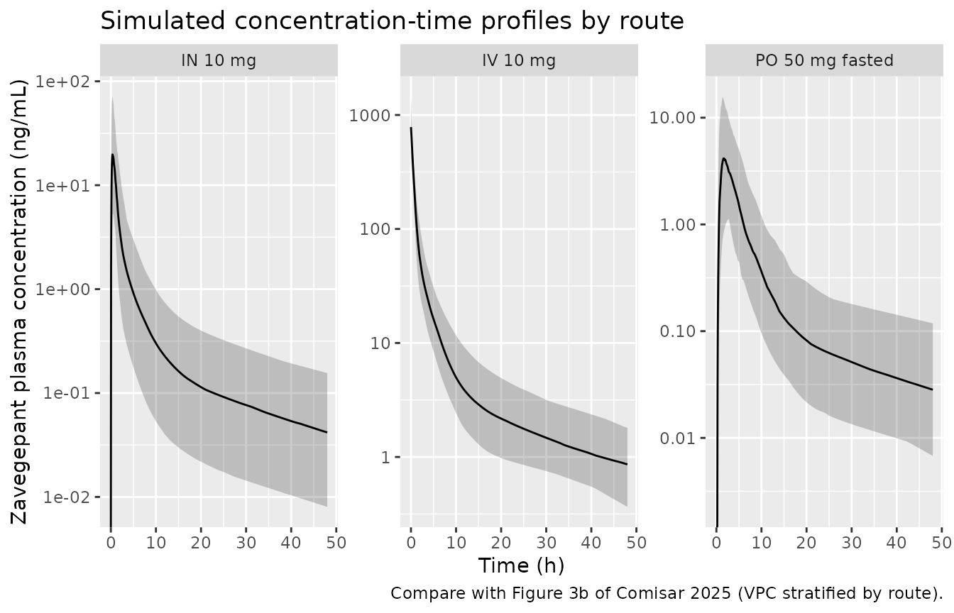

Allometric scaling (Discussion)

Comisar 2025 Discussion reports the population mean parameter ratios relative to the typical 70 kg individual at the 5th-percentile (57 kg) and highest (95 kg) body weights: clearance 85.7% and 126%, volume of distribution 81.4% and 136%. These are exact consequences of the fixed exponents and are reproduced here from the packaged model, not from the printed ratios.

allo_events <- tibble(
  id = 1:3, WT = c(57, 70, 95), ROUTE_ORAL = 0, FED = 0, HEPIMP_MOD = 0,
  CONMED_RIF = 0, CONMED_ITRACONAZOLE = 0
) |>
  mutate(time = 0, amt = 10, evid = 1L, rate = 0, cmt = "central") |>
  bind_rows(
    tibble(
      id = 1:3, WT = c(57, 70, 95), ROUTE_ORAL = 0, FED = 0, HEPIMP_MOD = 0,
      CONMED_RIF = 0, CONMED_ITRACONAZOLE = 0
    ) |>
      crossing(time = c(0.5, 1)) |>
      mutate(amt = NA_real_, evid = 0L, rate = 0, cmt = "central")
  ) |>
  arrange(id, time, desc(evid))

allo <- rxode2::rxSolve(rxode2::zeroRe(mod), events = allo_events,
                        keep = "WT") |>
  as.data.frame() |>
  group_by(WT) |>
  summarise(cl = first(cl), vc = first(vc), vp = first(vp), vp2 = first(vp2),
            .groups = "drop") |>
  mutate(vss = vc + vp + vp2)
#> ℹ parameter labels from comments will be replaced by 'label()'
#> ℹ omega/sigma items treated as zero: 'etalfdepot', 'etalka', 'etald1', 'etalvc', 'etalvp', 'etalcl'
#> Warning: multi-subject simulation without without 'omega'

ref <- allo |> filter(WT == 70)

allo_tab <- allo |>
  transmute(
    `Body weight (kg)`   = WT,
    `CL (L/h)`           = round(cl, 2),
    `CL vs 70 kg (%)`    = round(100 * cl / ref$cl, 1),
    `Vss (L)`            = round(vss, 1),
    `Vss vs 70 kg (%)`   = round(100 * vss / ref$vss, 1)
  )

knitr::kable(
  allo_tab,
  caption = paste(
    "Allometric scaling of the typical subject. Comisar 2025 Discussion reports",
    "CL 85.7% at 57 kg and 126% at 95 kg, and volume 81.4% and 136%."
  )
)

Allometric scaling of the typical subject. Comisar 2025 Discussion reports CL 85.7% at 57 kg and 126% at 95 kg, and volume 81.4% and 136%.
Body weight (kg)	CL (L/h)	CL vs 70 kg (%)	Vss (L)	Vss vs 70 kg (%)
57	11.40	85.7	72.3	81.4
70	13.30	100.0	88.8	100.0
95	16.72	125.7	120.5	135.7


# The published ratios are quoted to three significant figures, so match to
# 0.05 percentage points rather than merely "close".
stopifnot(
  abs(allo_tab$`CL vs 70 kg (%)`[allo_tab$`Body weight (kg)` == 57] - 85.7) < 0.05,
  abs(allo_tab$`CL vs 70 kg (%)`[allo_tab$`Body weight (kg)` == 95] - 125.7) < 0.05,
  abs(allo_tab$`Vss vs 70 kg (%)`[allo_tab$`Body weight (kg)` == 57] - 81.4) < 0.05,
  abs(allo_tab$`Vss vs 70 kg (%)`[allo_tab$`Body weight (kg)` == 95] - 135.7) < 0.05
)

# Typical Vss at 70 kg must be V2 + V3 + V4 = 12.1 + 66.0 + 10.7 = 88.8 L
# (Comisar 2025 Discussion).
stopifnot(abs(ref$vss - 88.8) < 1e-6)

The 95 kg CL ratio lands at 125.7%, which is the exact value of (95/70)^0.75; the paper rounds it to 126%. The 95 kg volume ratio is 135.7% against the paper’s 136%. Both are rounding, not disagreement.

Moderate hepatic impairment (Figure 2)

Comisar 2025 Figure 2 shows the distribution of relative mean exposure (AUC0-24 and Cmax) after a single 10 mg intranasal dose in participants with moderate hepatic impairment versus the reference population, with predicted mean increases of 63% and 12% respectively. The ratios below are typical-value predictions from the packaged model; the paper’s are medians of a distribution generated by sampling 3000 parameter sets from the variance-covariance matrix, so they are the comparable central estimates but not identical constructions.

hep_events <- bind_rows(
  make_arm("Normal hepatic function", 10, "depot", route_oral = 0,
           hepimp = 0, id_offset = 0L),
  make_arm("Moderate hepatic impairment", 10, "depot", route_oral = 0,
           hepimp = 1, id_offset = 100L)
) |>
  # Typical-value comparison: hold weight at the allometric reference so the
  # only difference between the arms is HEPIMP_MOD.
  mutate(WT = 70)

hep <- rxode2::rxSolve(rxode2::zeroRe(mod), events = hep_events,
                       keep = c("treatment", "HEPIMP_MOD")) |>
  as.data.frame()
#> ℹ parameter labels from comments will be replaced by 'label()'
#> ℹ omega/sigma items treated as zero: 'etalfdepot', 'etalka', 'etald1', 'etalvc', 'etalvp', 'etalcl'
#> Warning: multi-subject simulation without without 'omega'

hep_exposure <- hep |>
  filter(time <= 24) |>
  group_by(treatment) |>
  arrange(time, .by_group = TRUE) |>
  summarise(
    cmax     = max(Cc),
    auc_0_24 = sum(diff(time) * (head(Cc, -1) + tail(Cc, -1)) / 2),
    .groups  = "drop"
  )

hep_ratio <- tibble(
  Metric = c("AUC0-24", "Cmax"),
  `Simulated ratio (impaired / normal)` = c(
    hep_exposure$auc_0_24[hep_exposure$treatment == "Moderate hepatic impairment"] /
      hep_exposure$auc_0_24[hep_exposure$treatment == "Normal hepatic function"],
    hep_exposure$cmax[hep_exposure$treatment == "Moderate hepatic impairment"] /
      hep_exposure$cmax[hep_exposure$treatment == "Normal hepatic function"]
  ),
  `Comisar 2025 reported increase` = c("+63%", "+12%")
) |>
  mutate(`Simulated increase` = sprintf("%+.0f%%", 100 * (`Simulated ratio (impaired / normal)` - 1)),
         `Simulated ratio (impaired / normal)` = round(`Simulated ratio (impaired / normal)`, 3))

knitr::kable(
  hep_ratio,
  caption = paste(
    "Relative exposure in moderate hepatic impairment after a single 10 mg",
    "intranasal dose. Compare with Figure 2 of Comisar 2025."
  )
)

Relative exposure in moderate hepatic impairment after a single 10 mg intranasal dose. Compare with Figure 2 of Comisar 2025.
Metric	Simulated ratio (impaired / normal)	Comisar 2025 reported increase	Simulated increase
AUC0-24	1.651	+63%	+65%
Cmax	1.102	+12%	+10%


# The CL reduction is -43.9%, so the untruncated AUC ratio would be
# 1 / 0.561 = 1.783. AUC0-24 is truncated well before the terminal phase and
# must therefore sit strictly between 1 and that bound, near the paper's 1.63.
auc_ratio <- hep_ratio$`Simulated ratio (impaired / normal)`[hep_ratio$Metric == "AUC0-24"]
cmax_ratio <- hep_ratio$`Simulated ratio (impaired / normal)`[hep_ratio$Metric == "Cmax"]
stopifnot(auc_ratio > 1, auc_ratio < 1 / (1 - 0.439))
stopifnot(abs(auc_ratio - 1.63) < 0.15)
# Cmax is absorption-limited for a low-clearance compound given intranasally, so
# the clearance effect barely moves it.
stopifnot(cmax_ratio > 1, cmax_ratio < 1.25)

Food effect on oral bioavailability

Table 3 reports a -50.9% food effect on oral bioavailability, so the fed/fasted exposure ratio must be exactly 0.491 for otherwise-identical subjects. Because both oral arms were drawn with the same seed offsets but different random weights, this check is run on typical-value subjects.

food_events <- bind_rows(
  make_arm("PO 50 mg fasted", 50, "depot", route_oral = 1, fed = 0,
           id_offset = 0L),
  make_arm("PO 50 mg fed",    50, "depot", route_oral = 1, fed = 1,
           id_offset = 100L)
) |>
  mutate(WT = 70)

food <- rxode2::rxSolve(rxode2::zeroRe(mod), events = food_events,
                        keep = c("treatment", "FED")) |>
  as.data.frame()
#> ℹ parameter labels from comments will be replaced by 'label()'
#> ℹ omega/sigma items treated as zero: 'etalfdepot', 'etalka', 'etald1', 'etalvc', 'etalvp', 'etalcl'
#> Warning: multi-subject simulation without without 'omega'

food_ratio <- food |>
  group_by(treatment) |>
  arrange(time, .by_group = TRUE) |>
  summarise(auc = sum(diff(time) * (head(Cc, -1) + tail(Cc, -1)) / 2),
            .groups = "drop")

fed_fasted <- food_ratio$auc[food_ratio$treatment == "PO 50 mg fed"] /
  food_ratio$auc[food_ratio$treatment == "PO 50 mg fasted"]

# Bioavailability scales AUC linearly, so the ratio is the multiplier exactly.
stopifnot(abs(fed_fasted - (1 - 0.509)) < 1e-3)
cat(sprintf("Fed / fasted oral AUC ratio: %.4f (expected %.4f)\n",
            fed_fasted, 1 - 0.509))
#> Fed / fasted oral AUC ratio: 0.4910 (expected 0.4910)

PKNCA validation

sim_nca <- sim |>
  # Only !is.na(Cc): a `time > 0` or `Cc > 0` filter would drop the time-zero
  # row that PKNCA needs to anchor AUC.
  filter(!is.na(Cc)) |>
  select(id, time, Cc, treatment)

# Guarantee a time = 0 row per (id, treatment).
sim_nca <- bind_rows(
  sim_nca,
  sim_nca |> distinct(id, treatment) |> mutate(time = 0, Cc = 0)
) |>
  distinct(id, treatment, time, .keep_all = TRUE) |>
  arrange(id, treatment, time)

conc_obj <- PKNCA::PKNCAconc(sim_nca, Cc ~ time | treatment + id)

dose_df <- events |>
  filter(evid == 1) |>
  select(id, time, amt, treatment)

dose_obj <- PKNCA::PKNCAdose(dose_df, amt ~ time | treatment + id)

intervals <- data.frame(
  start      = 0,
  end        = Inf,
  cmax       = TRUE,
  tmax       = TRUE,
  aucinf.obs = TRUE,
  half.life  = TRUE
)

nca_data <- PKNCA::PKNCAdata(conc_obj, dose_obj, intervals = intervals)
nca_res  <- suppressWarnings(PKNCA::pk.nca(nca_data))

nca_wide <- as.data.frame(nca_res) |>
  select(treatment, id, PPTESTCD, PPORRES) |>
  pivot_wider(names_from = PPTESTCD, values_from = PPORRES)

nca_summary <- nca_wide |>
  group_by(treatment) |>
  summarise(
    n            = dplyr::n(),
    cmax_med     = median(cmax, na.rm = TRUE),
    tmax_med     = median(tmax, na.rm = TRUE),
    aucinf_med   = median(aucinf.obs, na.rm = TRUE),
    halflife_med = median(half.life, na.rm = TRUE),
    .groups      = "drop"
  )

nca_summary |>
  mutate(across(c(cmax_med, aucinf_med, halflife_med), \(x) signif(x, 3)),
         tmax_med = round(tmax_med, 2)) |>
  rename(
    "Arm"                       = treatment,
    "N"                         = n,
    "Cmax (ng/mL)"              = cmax_med,
    "Tmax (h)"                  = tmax_med,
    "AUC0-inf (ng*h/mL)"        = aucinf_med,
    "t1/2 (h)"                  = halflife_med
  ) |>
  knitr::kable(caption = "Median simulated NCA parameters by arm (PKNCA).")

Median simulated NCA parameters by arm (PKNCA).
Arm	N	Cmax (ng/mL)	Tmax (h)	AUC0-inf (ng*h/mL)	t1/2 (h)
IN 10 mg	100	21.70	0.40	35.4	21.0
IN 10 mg hepatic	100	22.60	0.45	51.3	25.2
IV 10 mg	100	783.00	0.00	727.0	22.0
PO 50 mg fasted	100	5.07	1.83	20.9	21.0
PO 50 mg fed	100	2.77	1.75	12.3	22.1

Per-subject mass-balance identity

Comisar 2025 reports no NCA parameter table, so there is no published Cmax / AUC to compare against directly. The stronger available check is the exact per-subject identity AUC0-inf = F * Dose / CL, which must hold for every individual in a linear model. Because fdepot and cl are returned as columns by rxSolve, this is testable without any tolerance on the population median (a median over 100 draws carries several percent of noise; the per-subject identity carries none).

per_subject <- sim |>
  group_by(id, treatment) |>
  summarise(cl = first(cl), fdepot = first(fdepot), .groups = "drop") |>
  left_join(
    events |> filter(evid == 1) |> select(id, amt),
    by = "id"
  ) |>
  left_join(nca_wide |> select(id, treatment, aucinf.obs),
            by = c("id", "treatment")) |>
  mutate(
    # IV doses go straight into `central`, so F = 1 for that arm; every other
    # arm passes through the depot and carries the route-specific F.
    f_applied = ifelse(treatment == "IV 10 mg", 1, fdepot),
    # amt is mg and cl is L/h, so amt/cl is mg*h/L; x1000 gives ng*h/mL.
    auc_expected = 1000 * f_applied * amt / cl,
    rel_error    = aucinf.obs / auc_expected - 1
  )

identity_tab <- per_subject |>
  group_by(treatment) |>
  summarise(
    n                    = dplyr::n(),
    `max |rel. error|`   = max(abs(rel_error), na.rm = TRUE),
    .groups              = "drop"
  )

identity_tab |>
  mutate(`max |rel. error|` = signif(`max |rel. error|`, 3)) |>
  rename("Arm" = treatment, "N" = n) |>
  knitr::kable(
    caption = paste(
      "Per-subject agreement between PKNCA AUC0-inf and F * Dose / CL.",
      "Residual error is numerical (observation-grid resolution and the",
      "log-linear extrapolation of the terminal tail), not structural."
    )
  )

Per-subject agreement between PKNCA AUC0-inf and F * Dose / CL. Residual error is numerical (observation-grid resolution and the log-linear extrapolation of the terminal tail), not structural.
Arm	N	max \|rel. error\|
IN 10 mg	100	0.00182
IN 10 mg hepatic	100	0.00073
IV 10 mg	100	0.00027
PO 50 mg fasted	100	0.00380
PO 50 mg fed	100	0.00122


# Fail loudly if the identity breaks for ANY subject in ANY arm. 2% accommodates
# the trapezoidal grid and terminal extrapolation only.
stopifnot(nrow(per_subject) == 5L * n_per_arm)
stopifnot(!anyNA(per_subject$rel_error))
stopifnot(max(abs(per_subject$rel_error)) < 0.02)

Comparison against published derived quantities

Comisar 2025 does not tabulate NCA results, but the Discussion derives several secondary quantities from the model. Those are reproduced here from the packaged model.

typ <- allo |> filter(WT == 70)
f_in <- exp(rxode2::rxode(mod)$theta[["lfdepot_intranasal"]])
#> ℹ parameter labels from comments will be replaced by 'label()'

derived <- tibble::tribble(
  ~Quantity,                                   ~Simulated,                         ~`Comisar 2025`,
  "Vss at 70 kg (L)",                          round(typ$vss, 1),                  88.8,
  "CL at 70 kg (L/h)",                         round(typ$cl, 1),                   13.3,
  "Apparent CL of intranasal zavegepant (L/h)", round(typ$cl / f_in, 0),           266,
  "Apparent Vss of intranasal zavegepant (L)",  round(typ$vss / f_in, 0),          1774
)

knitr::kable(
  derived,
  caption = paste(
    "Derived quantities from Comisar 2025 Discussion. The two apparent-parameter",
    "rows disagree by ~2% because the paper divided by an unrounded F of about",
    "5.0% while Table 3 prints 5.1%; see Assumptions and deviations."
  )
)

Derived quantities from Comisar 2025 Discussion. The two apparent-parameter rows disagree by ~2% because the paper divided by an unrounded F of about 5.0% while Table 3 prints 5.1%; see Assumptions and deviations.
Quantity	Simulated	Comisar 2025
Vss at 70 kg (L)	88.8	88.8
CL at 70 kg (L/h)	13.3	13.3
Apparent CL of intranasal zavegepant (L/h)	261.0	266.0
Apparent Vss of intranasal zavegepant (L)	1741.0	1774.0


# Vss and CL are exact; the apparent quantities inherit the paper's own
# F-rounding inconsistency and are checked only to that tolerance.
stopifnot(abs(typ$vss - 88.8) < 0.05, abs(typ$cl - 13.3) < 0.05)
stopifnot(abs(typ$cl / f_in / 266 - 1) < 0.03)
stopifnot(abs(typ$vss / f_in / 1774 - 1) < 0.03)

Assumptions and deviations

IIV convention. Comisar 2025 Table 3 reports inter-individual variability as “%IIV” with no footnote naming the convention. The values are read here as log-normal CV%, so omega^2 = log(CV^2 + 1) (the convention documented in the nlmixr2lib parameter-naming reference). The alternative reading omega^2 = CV^2 would give variances of 0.4369 (F), 0.1936 (ka), 1.3225 (D1), 0.1037 (Vc), 0.0681 (Vp) and 0.0718 (CL) instead of the values used. The two readings are close for every term except D1, whose 115% IIV maps to omega = 0.918 under the convention used here versus omega = 1.150 under the alternative. All typical-value results in this vignette are unaffected; only the width of the simulated variability bands changes.
Shared etas across routes. Each “%IIV” cell in Table 3 spans both the intranasal and the oral row of the quantity it belongs to, and the Methods list the evaluated IIV terms one-per-quantity rather than one-per-route (“bioavailability of intranasal and soft gelatin capsules”, etc.). A single eta is therefore shared between routes for F, ka and D1. Table 3 reports no off-diagonal covariances, so all etas are simulated independently.
Minutes converted to hours. D1 and the oral absorption lag are tabulated in minutes while the rest of the model is on an hours time base. They are divided by 60 here, which is what the paper does itself when it quotes “a D1 of 0.14 h” and “a D1 of 0.95 h” in the Results. The exact minute values are used rather than the paper’s two-significant-figure hour roundings.
Route encoding. ROUTE_ORAL was registered as a new canonical covariate column under the ROUTE_* family policy in inst/references/covariate-columns.md. Intravenous doses are distinguished from intranasal ones by the dose record’s cmt (they are placed directly into central) rather than by a second indicator column, so a single binary covariate covers the three-route design.
Rifampin route scope. Table 3 restricts the itraconazole clearance effect to oral zavegepant (“Co-administration of itraconazole on clearance when zavegepant administered orally”) but places no route restriction on the adjacent rifampin row, and the Discussion preserves exactly the same contrast – itraconazole “was not a significant covariate for intranasal zavegepant clearance, but decreased oral zavegepant clearance by 27.9%”, against a plain “Co-administration of rifampin … reduced zavegepant clearance by 41.1%”. The rifampin effect is therefore encoded here as route-independent.

Table 1 explains both why the two rows differ and why the choice is numerically moot. Study BHV3500-111 evaluated “the effects of rifampin on the pharmacokinetics of oral zavegepant and … the effects of itraconazole on the pharmacokinetics of zavegepant administered orally or as a nasal spray”. The dataset therefore contains no intranasal-plus-rifampin observations at all: the authors had no route contrast available to test for rifampin, so no restriction appears on that row, whereas for itraconazole they did have one, tested it, and found the effect only for oral. Because CONMED_RIF is never set on an intranasal or intravenous record in a dataset resembling the paper’s own, the route-independent and oral-restricted encodings give identical predictions there; they diverge only if a user deliberately simulates a combination the study never observed.

The paper’s prose is nonetheless inconsistent about this in three places. The Abstract says moderate hepatic impairment or rifampin “decreased elimination clearance of oral zavegepant by ~40%”; the Results covariate paragraph compresses the two DDIs into “co-administration of rifampin and itraconazole on CL of orally administered zavegepant (-41.1%, -27.9%)”; and the Study Highlights box says the same effects decreased clearance of “zavegepant nasal spray by ~40%”. The Abstract sentence is demonstrably unreliable on this point because it applies the same “oral” qualifier to moderate hepatic impairment, which the Discussion identifies as “the only clinically relevant covariate found for intranasal zavegepant administration” and which Figure 2 evaluates entirely on a 10 mg intranasal dose. Table 3 is the parameter source and is unambiguous.
Additive residual error units. Table 3 prints the fixed additive error as “0.001 ng/L” although the assay and the LLOQ (0.4 ng/mL) are in ng/mL. This is almost certainly a typo for ng/mL. Under either reading the term is a numerically negligible stabilising placeholder at least five orders of magnitude below the LLOQ, so it is entered as the printed 0.001 on the model’s ng/mL concentration scale and has no visible effect on any simulation.
Apparent-parameter arithmetic. The Discussion states that apparent intranasal clearance is “266 L/h (calculated by CL/intranasal bioavailability = 13.3 L/5.1%)”, but 13.3/0.051 = 260.8, not 266. Likewise 88.8/0.051 = 1741, not the quoted 1774. Both printed values correspond to dividing by an unrounded bioavailability of about 5.00%, so the underlying estimate was slightly below the 5.1% printed in Table 3. The tabulated 5.1% is used as the parameter here, and the derived-quantities check above is tolerated to 3% accordingly.
Female percentage conflict. Table 2 reports 126/277 (45.5%) female while the Results narrative states “female (49.3%)”. The Table 2 value is used in the model’s population metadata because it carries the underlying count.
Figure 1 compartment labels. The Figure 1 caption labels the two intercompartmental clearances Q2 and Q3, whereas Table 3 and the Results text label them Q3 and Q4. Table 3 and the Results agree with each other and with the volume labels V2/V3/V4, so that numbering is used; the mapping to nlmixr2lib names is V2 -> vc, V3 -> vp with Q3 -> q, and V4 -> vp2 with Q4 -> q2. Note that peripheral1 is the large slowly-equilibrating compartment (66.0 L at 2.6 L/h) and peripheral2 the small fast one (10.7 L at 5.2 L/h); this follows the paper’s numbering rather than a fast-then-slow convention.
Screened but unretained covariates. Age, sex, race, ethnicity, migraine status, creatinine clearance, oral contraceptives and sumatriptan were tested and not retained (Results “Covariate analysis”). Those with an existing canonical column are documented in the model’s covariatesDataExcluded metadata; they are deliberately absent from covariateData because the paper publishes no point estimate for any of them.
Supplement not on disk. Comisar 2025 cites Table S1 (bioanalytical method validation), Table S2 (covariates tested), Figure S1 (observed concentrations) and Figure S2 (external-validation VPC). None of these is on disk. None is a parameter source: Table 3 is complete, and every derived quantity quoted in the Discussion reproduces from it, so the extraction does not depend on the supplement.
Virtual cohort. Original observed data are not available. Body weight is drawn log-normally with median 74 kg truncated to the published 49-131 kg range; all other covariates are set to the arm definition rather than sampled, because the validation targets above are covariate-specific contrasts rather than population VPCs.
No non-paper-derived parameter values. Every ini() value comes from Comisar 2025 Table 3 or from the Methods statement of the fixed allometric exponents. No value was digitised from a figure, supplied by correspondence, or carried from an upstream model.