Ganciclovir and valganciclovir population-PK model repository (Yang 2023) • nlmixr2lib

Model and source

Yang 2023 is a PRISMA-registered systematic review that assembled a parametric population-PK model repository for ganciclovir (GCV) and its oral prodrug valganciclovir (VGCV). It identified 16 published population-PK models, replicated each in rxode2, ran a cross-model quality-control (QC) similarity comparison on four age-stratified typical virtual patients, compared covariate effects on clearance, and computed the probability of target attainment (PTA) for the commonly used dosing regimens.

The review is unusual among systematic reviews in that its Table 3 tabulates the complete fixed-effect equations, between-subject variability, and residual-error magnitude for every constituent model. That makes the review itself a usable extraction source, so the models below are transcribed from Yang 2023 Table 3 rather than skipped as a secondary source.

Article: https://doi.org/10.3390/pharmaceutics15071801
Yang 2023 supplementary materials (Tables S1-S2, Figures S1-S2, and the repository’s R source code) are hosted at https://www.mdpi.com/article/10.3390/pharmaceutics15071801/s1 and were not retrievable during extraction (the MDPI endpoint returns HTTP 403). Nothing in this vignette depends on them; see Assumptions and deviations.

Models contributed by this paper

All 11 of the review’s 16 models that were not already in nlmixr2lib are packaged here. The other five were already present, extracted directly from their primary publications, and are not re-extracted from the review (Caldes_2009_ganciclovir, Chen_2021_ganciclovir, Perrottet_2009_ganciclovir, Vezina_2010_valganciclovir, Vezina_2014_valganciclovir). Coverage of the review is therefore complete: 11 + 5 = 16.

Models extracted from Yang 2023 Table 3.
Model	Compartments	Route(s)	Population
Lalagkas_2023_ganciclovir	2	GCV IV + VGCV PO	Adult SOT recipients with CMV infection
Nguyen_2021_ganciclovir	2	GCV IV + VGCV PO	Pediatrics, incl. critically ill children
Franck_2021_ganciclovir	2	GCV IV + VGCV PO	Pediatric SOT and SCT recipients
Li_2021_ganciclovir	1	GCV IV	Critically ill children
Krens_2020_ganciclovir	1	GCV IV	Critically ill adults
Facchin_2019_ganciclovir	2	VGCV PO	Children with a renal transplant
Horvatits_2014_ganciclovir	2	GCV IV	Critically ill adults on CVVHDF
Zhao_2009_ganciclovir	2	VGCV PO	Pediatric renal transplant patients
Acosta_2007_ganciclovir	1	GCV IV + VGCV PO	Neonates with congenital CMV disease
Zhou_1996_ganciclovir	1	GCV IV	Newborns with congenital CMV disease
Yuen_1995_ganciclovir	2	GCV IV	CMV retinitis, CMV urine shedding, or SOT with renal dysfunction

Every model file records both citations – the primary publication and the Yang 2023 review it was transcribed from:

cat(rxode2::rxode2(readModelDb("Krens_2020_ganciclovir"))$reference)
#> ℹ parameter labels from comments will be replaced by 'label()'
#> Krens SD, Hodiamont CJ, Juffermans NP, Mathot RAA, van Hest RM. Population Pharmacokinetics of Ganciclovir in Critically Ill Patients. Ther Drug Monit. 2020;42(2):295-301. doi:10.1097/FTD.0000000000000689. Parameters transcribed from Yang W, Mak W, Gwee A, Gu M, Wu Y, Shi Y, He Q, Xiang X, Han B, Zhu X. Establishment and Evaluation of a Parametric Population Pharmacokinetic Model Repository for Ganciclovir and Valganciclovir. Pharmaceutics. 2023;15(7):1801. doi:10.3390/pharmaceutics15071801 (Table 3).

Population

The 11 packaged models were fitted to 11 separate cohorts published between 1995 and 2023, spanning newborns to adults. The table below reproduces the per-study demographics from Yang 2023 Table 2 (the review’s own tabulation of the primary studies).

Per-study demographics, from Yang 2023 Table 2. NR = not reported.
Study	Country	N	Observations	Age (median/mean)	Weight	Formulation
Lalagkas 2023	Spain	60	640	57 y (22-78)	68 kg (43-131)	GCV i.v. + VGCV p.o.
Nguyen 2021	France	105	374	2.5 y (0.01-17.3)	11.7 kg (2.6-80)	GCV i.v. + VGCV p.o.
Franck 2021	Canada	50	580	7.5 y (0.5-17.4)	26.7 kg (5.96-87)	GCV i.v. + VGCV p.o.
Li 2021	China	104	138	2.46 y (0.10-12.83)	12.0 kg (2.5-55.0)	GCV i.v.
Krens 2020	Netherlands	34	128	56 y (30-82)	70 kg (44-140)	GCV i.v.
Facchin 2019	France	104	1212	12.2 y (2.1-20.5)	30.35 kg (11.9-83.0)	VGCV p.o.
Horvatits 2014	see note	9	NR	56 +/- 9 y	86 +/- 25 kg	GCV i.v.
Zhao 2009	France	22	164	9 y (3-17)	28 kg (12-76)	VGCV p.o.
Acosta 2007	USA	24	484	30 d (11-34) / 20 d (8-33)	2.7 / 2.9 kg	GCV i.v. + VGCV p.o.
Zhou 1996	USA	27	219	Newborns	NR	GCV i.v.
Yuen 1995	USA	53	558	NR	NR	GCV i.v.

Yang 2023 Table 2 lists the Horvatits 2014 country as “Australia”; the Horvatits 2014 author group is Vienna-based, so this is flagged in that model’s population$regions as a probable transcription error in the review, to be resolved against the primary publication.

The same information is available programmatically per model, e.g. rxode2::rxode2(readModelDb("Franck_2021_ganciclovir"))$population.

Across the 16 reviewed models the review found (Yang 2023 Sections 3.3.3, 4.3): body size (weight or BSA) was a significant covariate on CL in 9/16 studies, and renal function (eGFR, CLcr, or serum creatinine) in 13/16 – every one of which produced a clinically significant (>20%) change in CL over the covariate’s normal range. Sex reached significance in only two studies and was not clinically meaningful.

Source trace

Per-parameter provenance is recorded as an in-file comment next to each ini() line in inst/modeldb/specificDrugs/<model>.R. Every structural parameter, between-subject variance, and residual-error term in all 11 models comes from a single source location: Yang 2023 Table 3 (“Model strategies and final pharmacokinetic parameters of the included studies”), in the row for that study – with the group-effect coefficients of Nguyen_2021 and Yuen_1995 defined in Table 3’s own footnote. The table below collects the structural equations exactly as Table 3 prints them.

Model	Fixed-effect equations (verbatim from Yang 2023 Table 3)	BSV (%)	RUV
`Lalagkas_2023`	CL = 6.93 x (CKD-EPI/55)^0.817 x (BW/70)^0.75; Vc = 43.1 x (BW/70); Q = 9.23 x (BW/70)^0.75; Vp = 219 x (BW/70); Ka = 0.766; F = 0.699; Tlag = 0.331	CL 29.9, Vc 36.1, Vp 103.4, Ka 45.7, F 16.6	28.2% prop + 0.237 mg/L add
`Nguyen_2021`	CL = 2.55 x (BW/11.7)^0.75 x (eGFR/167)^0.763 x 0.806^critically ill; Vc = 5.96 x (BW/11.7); Q = 0.222 x (BW/11.7)^0.75; Vp = 1.29 x (BW/11.7); Ka = 0.506; F = 0.438	CL 48.6, Vc 46.9	47.7% prop
`Franck_2021`	CL = 6.9 x (BW/26.7)^0.75 x (CrCL/149.8)^0.88; Vc = 9.7 x (BW/26.7); Q = 10.9; Vp = 7.6 x (BW/26.7); Tlag = 0.33; Ka = 0.73; F = 0.43	CL 66.3, Vc 76.8, Ka 83.7, F 55.7	0.98 mg/L add
`Li_2021`	CL = 5.23 x KF^0.92 x (BW/12.0)^1.02, KF = eGFR/120; Vc = 11.35 x (BW/12.0)^0.80	CL 12.9, Vc 65.8	8.23% prop
`Krens_2020`	CL = 2.3 x (CKD-EPI/65)^0.71; Vc = 42	CL 47.0, Vc 80.0	43% prop
`Facchin_2019`	CL/F = 9.07 x (SCR/72.5)^-0.768 x BSA^1.31 x 1.15^GENDER; Vc/F = 45 x BSA^1.28 x 1.14^GENDER; Q/F = 1.46; Vp/F = 18.5; Ka = 6.96; Tlag = 0.86	CL 16.0, Vc 9.3, Vp 54.6, Ka 59.2	23.5% prop
`Horvatits_2014`	CL = 2.2; Vc = 32.4; Q = 16.8; Vp = 33.5	CL 61.5, Vc 33.6, Q 34.7, Vp 60.6	7.22% prop
`Zhao_2009`	CL/F = 8.04 x (CLcr/89)^2.93 + 3.62 x (BW/28); Vc/F = 5.2; Vp/F = 30.7; Q/F = 3.97; Ka = 0.369; Tlag = 0.743	CL 23.83, Vc 58.22, Ka 32.25	20.93% exponential
`Acosta_2007`	CL = 0.146 x BW^1.68; V = 1.15 x BW; Ka = 0.591; F = 0.536	CL 28.4, F 12.4	45.4% exponential
`Zhou_1996`	CL = 0.262 + (0.00271 x ASCC); Vc = 0.627 + (0.437 x BW)	CL 35.4, Vc 30.1, COV 28.5	8.46% prop
`Yuen_1995`	CL = 0.382 + 0.168 x BW x CLcr/100 x (1-T) x (1-CMV); Vc = 0.381 x BW; Vp = 0.511 x BW; Q = 13.4	CL 47.5, Vc 27.5	36.1% prop

Supporting source locations for the encoding conventions:

Convention	Source location
`Nguyen_2021` critical-illness coding (1 = critically ill, 0 = others)	Yang 2023 Table 3 footnote: “critically ill: 1 for critically ill patients and 0 for others”
`Yuen_1995` transplant coefficient T = 0.76 (0 for non-transplant)	Yang 2023 Table 3 footnote: “T: T = 0 for non-transplant patients and 0.76 for transplant patients”
`Yuen_1995` CMV coefficient 0.41 (0 for CMV-shedding, 0.41 for retinitis)	Yang 2023 Table 3 footnote: “CMV: CMV = 0 for CMV-shedding patients and 0.41 for patients with CMV retinitis”
BSV reported as %CV with omega = %CV/100 (so variance = (%CV/100)^2)	Yang 2023 Section 2.2: “BSV … was recorded as the coefficient of variation (CV), and %CV = sqrt(omega^2) * 100%”
BSV is exponential in every included study	Yang 2023 Section 3.2.1: “BSV was described by an exponential model in all the included studies.”
Exponential residual error encoded as proportional in linear space	Yang 2023 Section 3.2.1 residual-error tabulation; exponential residual on the natural scale = additive on the log scale = `prop()` in nlmixr2
Absorption of VGCV is first-order in every related study	Yang 2023 Section 3.2.1: “Absorption of VGCV in all related studies was described as a first-order absorption process.”
Lalagkas 2023 and Caldes 2009 converted VGCV doses to GCV equivalents (x 0.72)	Yang 2023 Section 3.2.1 and Table 3 footnote `*`
Covariate units (CKD-EPI, CrCL, CLcr, ASCC, SCR, BSA, GENDER coding)	Yang 2023 Table 3 footnote
Covariates tested vs retained per study	Yang 2023 Table 4
Facchin 2019 IOV (CL 14.4%, Vp 77.2%, ka 111.4%) – omitted per registry convention	Yang 2023 Section 3.2.1
Typical virtual patients (age, weight, height, SCR)	Yang 2023 Table 1
QC acceptance band (50-200%; achieved 70-150%)	Yang 2023 Sections 2.3 and 3.3.1
PTA targets (40-80, 80-120, >120 mg*h/L)	Yang 2023 Sections 2.5.1 and 3.4.1

Virtual cohort

Original observed data are not publicly available. Yang 2023 Section 2.3 built four age-stratified typical virtual patients (Table 1) and simulated 1000 subjects per model per patient; the simulations below reproduce that design with 80 subjects per arm (well inside the 200-per-arm cap, and ample for the geometric-mean comparison the review’s QC criterion is based on).

Yang 2023 Table 1 gives age, weight, height, and serum creatinine for each virtual patient but not the derived body surface area or renal function that several models require; those live in the unavailable Table S1. They are derived here with standard formulas, documented in Assumptions and deviations.

set.seed(20260729)

# Yang 2023 Table 1 -- typical virtual patients (all male).
vp <- tibble::tribble(
  ~cohort,     ~age_label,     ~WT, ~HT,  ~CREAT,
  "Neonates",  "40 wk PMA",      3,  50,      30,
  "Infants",   "1 year",        10,  70,      50,
  "Children",  "10 years",      30, 130,      70,
  "Adults",    "40 years",      70, 170,      95
) |>
  mutate(
    SEXF = 0,                                   # all male (Yang 2023 Table 1)
    # Mosteller BSA (m^2)
    BSA  = sqrt(HT * WT / 3600),
    # Serum creatinine umol/L -> mg/dL
    creat_mgdl = CREAT / 88.4,
    # Renal function, BSA-normalized (mL/min/1.73 m^2):
    #  - pediatric cohorts: bedside Schwartz, 0.413 * height(cm) / SCr(mg/dL)
    #  - adult cohort: Cockcroft-Gault, then normalized to 1.73 m^2
    crcl_norm = ifelse(
      cohort == "Adults",
      ((140 - 40) * WT / (72 * creat_mgdl)) * 1.73 / BSA,
      0.413 * HT / creat_mgdl
    ),
    # Raw (un-normalized) creatinine clearance, mL/min
    crcl_raw = crcl_norm * BSA / 1.73
  )

vp |>
  transmute(
    "Cohort"                  = cohort,
    "Age"                     = age_label,
    "Weight (kg)"             = WT,
    "Height (cm)"             = HT,
    "SCr (umol/L)"            = CREAT,
    "BSA (m^2)"               = round(BSA, 3),
    "eGFR (mL/min/1.73 m^2)"  = round(crcl_norm, 1),
    "CrCl (mL/min)"           = round(crcl_raw, 1)
  ) |>
  knitr::kable(caption = "Yang 2023 Table 1 virtual patients (first five columns) plus derived BSA and renal function.")

Yang 2023 Table 1 virtual patients (first five columns) plus derived BSA and renal function.
Cohort	Age	Weight (kg)	Height (cm)	SCr (umol/L)	BSA (m^2)	eGFR (mL/min/1.73 m^2)	CrCl (mL/min)
Neonates	40 wk PMA	3	50	30	0.204	60.8	7.2
Infants	1 year	10	70	50	0.441	51.1	13.0
Children	10 years	30	130	70	1.041	67.8	40.8
Adults	40 years	70	170	95	1.818	86.1	90.5

Arms

Each model is simulated only in the age cohort(s) its source study targeted, and only via the route(s) it can support. Models parameterized in apparent oral clearances (Facchin_2019, Zhao_2009) are oral-only; models without a depot compartment (Li_2021, Krens_2020, Horvatits_2014, Zhou_1996) are IV-only. Yuen_1995’s cohort has no reported weights or ages but was an adult population (CMV retinitis, CMV urine shedding, and solid-organ transplant recipients), so it is simulated in the adult cohort, IV-only.

# `crcl_kind` selects which renal-function variant the model's CRCL column means
# (Yang 2023 Table 3 footnote distinguishes CrCL / eGFR / CKD-EPI / ASCC in
# mL/min/1.73 m^2 from CLcr in raw mL/min).
arms <- tibble::tribble(
  ~model,                        ~cohort,     ~route,     ~crcl_kind,
  "Zhou_1996_ganciclovir",       "Neonates",  "GCV IV",   "norm",
  "Acosta_2007_ganciclovir",     "Neonates",  "GCV IV",   "norm",
  "Acosta_2007_ganciclovir",     "Neonates",  "VGCV PO",  "norm",
  "Franck_2021_ganciclovir",     "Infants",   "GCV IV",   "norm",
  "Franck_2021_ganciclovir",     "Children",  "GCV IV",   "norm",
  "Franck_2021_ganciclovir",     "Infants",   "VGCV PO",  "norm",
  "Franck_2021_ganciclovir",     "Children",  "VGCV PO",  "norm",
  "Nguyen_2021_ganciclovir",     "Infants",   "GCV IV",   "norm",
  "Nguyen_2021_ganciclovir",     "Children",  "GCV IV",   "norm",
  "Nguyen_2021_ganciclovir",     "Infants",   "VGCV PO",  "norm",
  "Nguyen_2021_ganciclovir",     "Children",  "VGCV PO",  "norm",
  "Li_2021_ganciclovir",         "Infants",   "GCV IV",   "norm",
  "Li_2021_ganciclovir",         "Children",  "GCV IV",   "norm",
  "Facchin_2019_ganciclovir",    "Children",  "VGCV PO",  "norm",
  "Zhao_2009_ganciclovir",       "Children",  "VGCV PO",  "raw",
  "Lalagkas_2023_ganciclovir",   "Adults",    "GCV IV",   "norm",
  "Lalagkas_2023_ganciclovir",   "Adults",    "VGCV PO",  "norm",
  "Krens_2020_ganciclovir",      "Adults",    "GCV IV",   "norm",
  "Horvatits_2014_ganciclovir",  "Adults",    "GCV IV",   "norm",
  "Yuen_1995_ganciclovir",       "Adults",    "GCV IV",   "raw"
) |>
  mutate(
    study = sub("_ganciclovir$", "", model),
    arm   = paste(study, cohort, route, sep = " | ")
  )

nrow(arms)
#> [1] 20

Simulation

Dosing follows Yang 2023 Section 2.3: all virtual patients receive GCV 5 mg/kg by 1-hour IV infusion q12h; for VGCV, neonates / infants / children receive 10 mg/kg q12h and adults 900 mg q12h. Lalagkas_2023 converted VGCV doses to ganciclovir equivalents (x 0.72), so its oral dose is scaled accordingly.

Eight doses are given (0, 12, …, 84 h), with the first carrying ss = 1 and ii = 12 so that rxode2 starts the system at the analytic steady state of the q12h regimen rather than accumulating toward it. This is load-bearing: the slowest models here have terminal half-lives above 30 h, so a dose-from-zero run would still be accumulating at 72 h and every “steady-state” exposure would be biased low. Observation continues to 168 h, so the 72-96 h window is a true steady-state 24-hour interval (two dosing intervals, matching the review’s AUC0-24h endpoint) and 84-168 h is a clean 84-hour washout for terminal half-life.

n_per_arm <- 80L
tau       <- 12
dose_times <- seq(0, 84, by = tau)

obs_grid <- sort(unique(c(
  seq(0,   72, by = 4),
  seq(72,  96, by = 0.25),
  seq(96, 168, by = 1)      # washout after the final 84 h dose, for terminal t1/2
)))

# GCV-equivalent oral dose factor: only the studies that converted VGCV doses.
vgcv_to_gcv <- c("Lalagkas_2023_ganciclovir" = 0.72)

make_arm_events <- function(model, cohort, route, crcl_kind, arm, id_offset) {
  pat <- vp[vp$cohort == cohort, ]
  ids <- id_offset + seq_len(n_per_arm)

  crcl <- if (crcl_kind == "raw") pat$crcl_raw else pat$crcl_norm

  subj <- tibble(
    id    = ids,
    WT    = pat$WT,
    BSA   = pat$BSA,
    CREAT = pat$CREAT,
    SEXF  = pat$SEXF,
    CRCL  = crcl,
    # Three group indicators are each set to their model's REFERENCE category, so
    # every arm reports that model's typical-value profile and the cross-model QC
    # comparison is not confounded by a subgroup shift. The non-reference levels
    # are exercised separately in the covariate-effect section below.
    #   DIS_CRITILL       (Nguyen_2021): 0 = not critically ill
    #   TX_ANY            (Yuen_1995):   0 = non-transplant patient
    #   DIS_CMV_RETINITIS (Yuen_1995):   0 = CMV-positive without retinitis
    #                                        (asymptomatic urine shedding)
    DIS_CRITILL       = 0,
    TX_ANY            = 0,
    DIS_CMV_RETINITIS = 0,
    arm   = arm,
    cohort = cohort,
    route  = route
  )

  if (route == "GCV IV") {
    amt_mg  <- 5 * pat$WT             # 5 mg/kg
    dose_cmt <- "central"
    dur_h    <- 1                     # 1-hour infusion
  } else {
    amt_vgcv <- if (cohort == "Adults") 900 else 10 * pat$WT
    amt_mg   <- amt_vgcv * unname(ifelse(model %in% names(vgcv_to_gcv), vgcv_to_gcv[model], 1))
    dose_cmt <- "depot"
    dur_h    <- 0                     # oral: instantaneous input into depot
  }

  # The first dose record carries ss = 1 with ii = tau, so rxode2 initialises the
  # system at the ANALYTIC steady state of the q12h regimen. This matters: the
  # slowest models here have a terminal half-life above 30 h, so a
  # dose-from-zero run would still be accumulating at 72 h and the "steady-state"
  # AUC would be biased low. The remaining explicit doses then carry the profile
  # forward so the final dose can be followed by a real washout.
  dose_rows <- tidyr::expand_grid(id = ids, time = dose_times) |>
    mutate(
      amt      = amt_mg,
      cmt      = dose_cmt,
      evid     = 1L,
      rate     = if (dur_h > 0) amt_mg / dur_h else 0,
      duration = dur_h,
      ss       = ifelse(time == 0, 1L, 0L),
      ii       = ifelse(time == 0, tau, 0)
    )

  obs_rows <- tidyr::expand_grid(id = ids, time = obs_grid) |>
    mutate(amt = 0, cmt = "central", evid = 0L, rate = 0, duration = 0,
           ss = 0L, ii = 0)

  bind_rows(dose_rows, obs_rows) |>
    left_join(subj, by = "id") |>
    arrange(id, time, desc(evid))
}

# Solve each model once, over all of its arms.
sim_list <- list()
for (m in unique(arms$model)) {
  m_arms <- arms[arms$model == m, ]
  ev <- dplyr::bind_rows(lapply(seq_len(nrow(m_arms)), function(i) {
    make_arm_events(
      model     = m_arms$model[i],
      cohort    = m_arms$cohort[i],
      route     = m_arms$route[i],
      crcl_kind = m_arms$crcl_kind[i],
      arm       = m_arms$arm[i],
      id_offset = (which(arms$arm == m_arms$arm[i]) - 1L) * 1000L
    )
  }))

  mod <- readModelDb(m)
  s <- rxode2::rxSolve(
    mod, events = ev,
    keep = c("arm", "cohort", "route", "WT", "CRCL"),
    useLinCmt = FALSE
  )
  sim_list[[m]] <- as.data.frame(s) |> mutate(model = m)
}
#> ℹ parameter labels from comments will be replaced by 'label()'
#> ℹ parameter labels from comments will be replaced by 'label()'
#> ℹ parameter labels from comments will be replaced by 'label()'
#> ℹ parameter labels from comments will be replaced by 'label()'
#> ℹ parameter labels from comments will be replaced by 'label()'
#> ℹ parameter labels from comments will be replaced by 'label()'
#> ℹ parameter labels from comments will be replaced by 'label()'
#> ℹ parameter labels from comments will be replaced by 'label()'
#> ℹ parameter labels from comments will be replaced by 'label()'
#> ℹ parameter labels from comments will be replaced by 'label()'
#> ℹ parameter labels from comments will be replaced by 'label()'
sim <- dplyr::bind_rows(sim_list)

# Sanity: every arm produced non-missing concentrations.
stopifnot(nrow(sim) > 0)
stopifnot(all(sort(unique(sim$arm)) == sort(unique(arms$arm))))
stopifnot(all(tapply(sim$Cc, sim$arm, function(x) any(is.finite(x) & x > 0))))

Replicate published figures

Figures 2 and 3 – steady-state concentration-time profiles by age group

Yang 2023 Figure 2 (IV ganciclovir) and Figure 3 (oral valganciclovir) show simulated steady-state profiles for neonates, infants, children, and adults, with the median and 10th-90th percentiles across the virtual population, one line per retrieved study. The panels below reproduce that layout over the 72-96 h steady-state window for the 11 packaged models.

prof <- sim |>
  filter(time >= 72, time <= 96) |>
  mutate(time_ss = time - 72) |>
  group_by(model, arm, cohort, route, time_ss) |>
  summarise(
    Q10 = quantile(Cc, 0.10, na.rm = TRUE),
    Q50 = quantile(Cc, 0.50, na.rm = TRUE),
    Q90 = quantile(Cc, 0.90, na.rm = TRUE),
    .groups = "drop"
  ) |>
  mutate(
    study  = sub("_ganciclovir$", "", model),
    cohort = factor(cohort, levels = c("Neonates", "Infants", "Children", "Adults"))
  )

ggplot(prof, aes(time_ss, Q50, colour = study, fill = study)) +
  geom_ribbon(aes(ymin = Q10, ymax = Q90), alpha = 0.15, colour = NA) +
  geom_line(linewidth = 0.7) +
  facet_grid(cohort ~ route, scales = "free_y") +
  labs(
    x = "Time within steady-state 24 h window (h)",
    y = "Ganciclovir concentration (mg/L)",
    colour = "Study", fill = "Study",
    title = "Replicates Yang 2023 Figures 2 (GCV IV) and 3 (VGCV PO)",
    caption = paste(
      "Line: simulated median. Band: 10th-90th percentile.",
      "GCV 5 mg/kg q12h 1 h IV infusion; VGCV 10 mg/kg q12h (pediatric) or 900 mg q12h (adult)."
    )
  ) +
  theme_bw() +
  theme(legend.position = "bottom")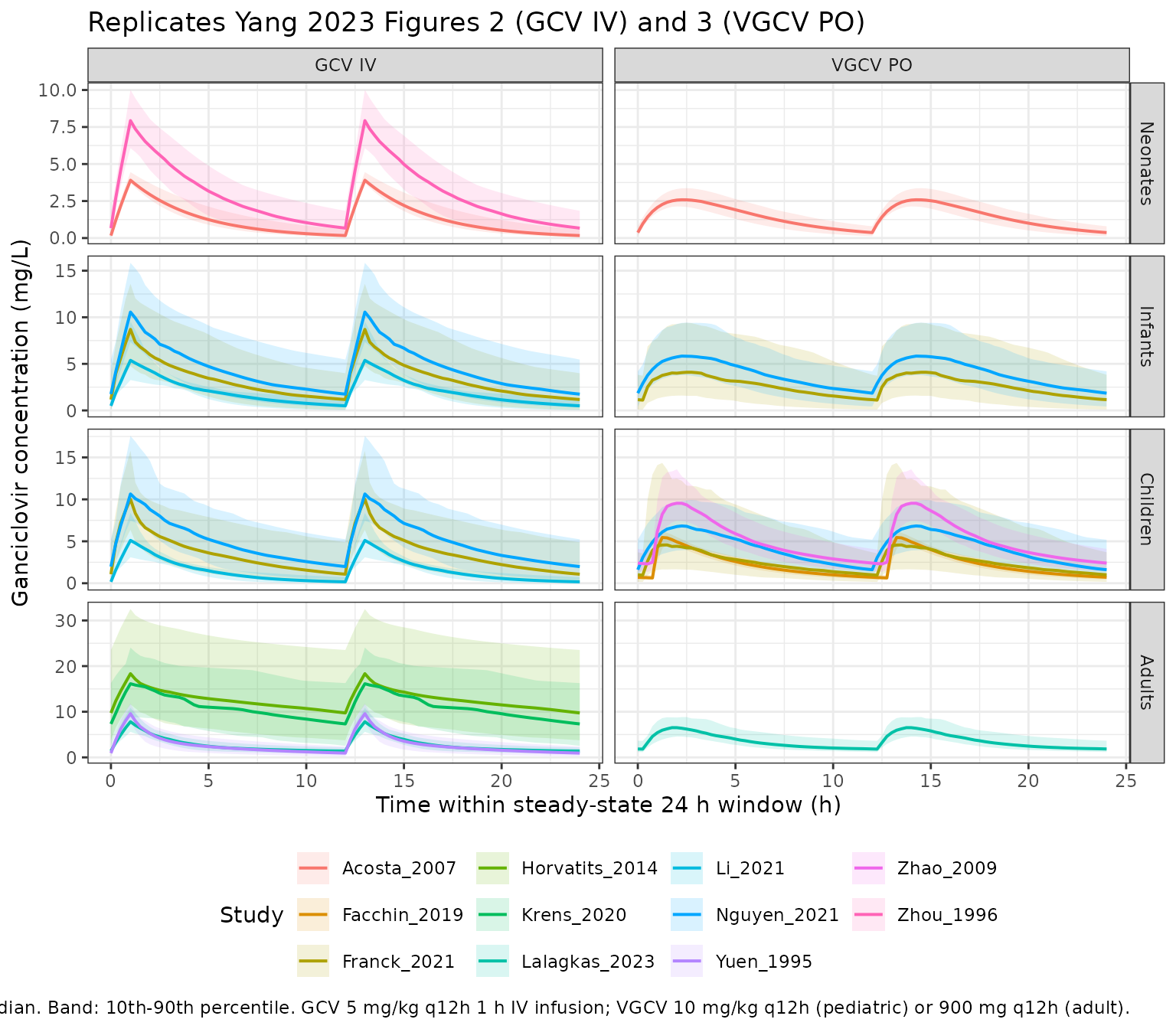

Consistent with Yang 2023 Sections 3.3.2 and 4.1, the pediatric profiles are broadly comparable across models (weight-based dosing largely resolves between-cohort PK differences), while the adult profiles separate: the two critically ill adult models (Krens_2020, Horvatits_2014) sit well above Lalagkas_2023 at the same 5 mg/kg dose.

Figure 4 – covariate effect on clearance

Yang 2023 Figure 4 is a forest plot of each study’s covariate effect on CL, expressed as the ratio of CL across the covariate’s range to the typical CL, with a shaded 0.8-1.25 “clinically insignificant” band. The equivalent computation for the renal-function and body-size effects of the packaged models:

# Renal-function effect: CL ratio between the low and high end of a common
# eGFR range (Yang 2023 scaled renal function to a uniform range; the exact
# Table S1 endpoints are unavailable, so 30-130 mL/min/1.73 m^2 is used).
# `Zhao_2009` and `Yuen_1995` use raw CLcr in mL/min rather than the normalized
# scale; the two coincide to within the BSA ratio (~5% for a 70 kg adult), which
# is far smaller than the effect sizes being plotted, so the same range is used
# for every model to keep the comparison on one axis (as Yang 2023 Figure 4 does).
renal_lo <- 30; renal_hi <- 130
ref_norm <- 90   # reference renal function for the ratio

# `additive_yuen` evaluates Yuen 1995's CL = 0.382 + 0.168 * BW * CLcr/100 at a
# 70 kg adult (the cohort weights are not reported), so its renal term is the
# dominant one and the ratio is close to -- but not exactly -- proportional.
yuen_cl <- function(crcl, wt = 70) 0.382 + 0.168 * wt * crcl / 100

renal_effects <- tibble::tribble(
  ~study,           ~ref,   ~expo,   ~kind,
  "Lalagkas_2023",  55,     0.817,   "power",
  "Nguyen_2021",    167,    0.763,   "power",
  "Franck_2021",    149.8,  0.88,    "power",
  "Li_2021",        120,    0.92,    "power",
  "Krens_2020",     65,     0.71,    "power",
  "Zhao_2009",      89,     2.93,    "power_partial",
  "Zhou_1996",      NA,     NA,      "additive",
  "Yuen_1995",      NA,     NA,      "additive_yuen"
) |>
  rowwise() |>
  mutate(
    cl_lo = dplyr::case_when(
      kind == "power"         ~ (renal_lo / ref)^expo,
      kind == "power_partial" ~ (8.04 * (renal_lo / ref)^expo + 3.62) / (8.04 + 3.62),
      kind == "additive"      ~ (0.262 + 0.00271 * renal_lo) / (0.262 + 0.00271 * ref_norm),
      kind == "additive_yuen" ~ yuen_cl(renal_lo) / yuen_cl(ref_norm)
    ),
    cl_hi = dplyr::case_when(
      kind == "power"         ~ (renal_hi / ref)^expo,
      kind == "power_partial" ~ (8.04 * (renal_hi / ref)^expo + 3.62) / (8.04 + 3.62),
      kind == "additive"      ~ (0.262 + 0.00271 * renal_hi) / (0.262 + 0.00271 * ref_norm),
      kind == "additive_yuen" ~ yuen_cl(renal_hi) / yuen_cl(ref_norm)
    ),
    cl_ref = dplyr::case_when(
      kind == "power"         ~ (ref_norm / ref)^expo,
      kind == "power_partial" ~ (8.04 * (ref_norm / ref)^expo + 3.62) / (8.04 + 3.62),
      kind == "additive"      ~ 1,
      kind == "additive_yuen" ~ 1
    )
  ) |>
  ungroup() |>
  mutate(across(c(cl_lo, cl_hi), ~ .x / cl_ref))

ggplot(renal_effects, aes(y = study)) +
  annotate("rect", xmin = 0.8, xmax = 1.25, ymin = -Inf, ymax = Inf,
           fill = "grey80", alpha = 0.6) +
  geom_vline(xintercept = 1, linetype = "dashed") +
  geom_segment(aes(x = cl_lo, xend = cl_hi, yend = study), linewidth = 1.2) +
  geom_point(aes(x = cl_lo)) +
  geom_point(aes(x = cl_hi)) +
  scale_x_log10() +
  labs(
    x = sprintf("CL ratio vs. reference, renal function %g-%g mL/min/1.73 m^2",
                renal_lo, renal_hi),
    y = NULL,
    title = "Replicates Yang 2023 Figure 4 (renal-function effect on CL)",
    caption = "Shaded band: 0.8-1.25 (Yang 2023 clinical-significance boundary)."
  ) +
  theme_bw()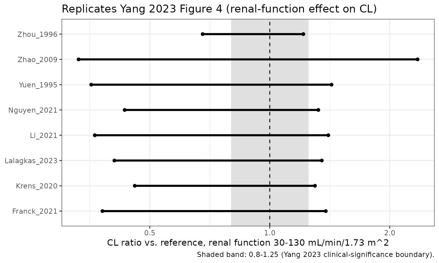

Every packaged model’s renal-function effect falls outside the 0.8-1.25 band, reproducing Yang 2023 Section 4.3: “regardless of the renal function indicator (i.e., eGFR, CLcr, SCR), the covariate effect on CL was clinically significant.” The Zhao_2009 bar is by far the widest – a direct consequence of the CLcr exponent of 2.93 printed in Table 3, which is flagged below.

PKNCA validation

nca_conc <- sim |>
  filter(!is.na(Cc)) |>
  select(id, time, Cc, arm, cohort, route, model)

# Rebuild the dose records for PKNCA from the same generator used for solving.
dose_records <- dplyr::bind_rows(lapply(seq_len(nrow(arms)), function(i) {
  make_arm_events(
    model     = arms$model[i],
    cohort    = arms$cohort[i],
    route     = arms$route[i],
    crcl_kind = arms$crcl_kind[i],
    arm       = arms$arm[i],
    id_offset = (i - 1L) * 1000L
  ) |>
    filter(evid == 1L) |>
    select(id, time, amt, duration, arm, cohort, route)
}))

conc_obj <- PKNCA::PKNCAconc(
  nca_conc, Cc ~ time | arm + id,
  concu = "mg/L", timeu = "hr"
)
#> Warning in assert_conc(conc, any_missing_conc = any_missing_conc): Negative
#> concentrations found
dose_obj <- PKNCA::PKNCAdose(
  dose_records, amt ~ time | arm + id,
  duration = "duration", doseu = "mg"
)
#> Found column named route, using it for the attribute of the same name.

arm_levels <- sort(unique(arms$arm))

# Three windows, each scoped to the endpoint it can actually define:
#  1. 72-96 h  -- AUC0-24h at steady state (the review's exposure endpoint;
#                 deliberately spans the two q12h dosing intervals of a 24 h day).
#  2. 84-96 h  -- ONE dosing interval (tau = 12 h), for Cmax / Tmax / Cmin / Cav.
#                 Tmax and Cmin are undefined over a two-dose window: at steady
#                 state the peaks after the 72 h and 84 h doses are numerically
#                 near-identical, so Cmax lands after either one essentially at
#                 random and a summary of Tmax over 72-96 h is a meaningless
#                 average of a bimodal quantity (~1 h vs ~13 h).
#  3. 84-168 h -- the 84 h washout after the final dose, for terminal half-life.
intervals <- bind_rows(
  tibble(arm = arm_levels, start = 72, end = 96,
         cmax = FALSE, tmax = FALSE, cmin = FALSE, auclast = TRUE, cav = FALSE,
         half.life = FALSE),
  tibble(arm = arm_levels, start = 84, end = 96,
         cmax = TRUE, tmax = TRUE, cmin = TRUE, auclast = FALSE, cav = FALSE,
         half.life = FALSE),
  tibble(arm = arm_levels, start = 84, end = 168,
         cmax = FALSE, tmax = FALSE, cmin = FALSE, auclast = FALSE, cav = FALSE,
         half.life = TRUE)
)

nca_res <- suppressWarnings(
  PKNCA::pk.nca(PKNCA::PKNCAdata(conc_obj, dose_obj, intervals = intervals))
)
nca_tbl <- as.data.frame(nca_res$result)

head(nca_tbl, 4)
#>                             arm id start end PPTESTCD     PPORRES exclude
#> 1 Zhou_1996 | Neonates | GCV IV  1    72  96  auclast 40.33303180    <NA>
#> 2 Zhou_1996 | Neonates | GCV IV  1    84  96     cmax  8.51343539    <NA>
#> 3 Zhou_1996 | Neonates | GCV IV  1    84  96     cmin  0.02085064    <NA>
#> 4 Zhou_1996 | Neonates | GCV IV  1    84  96     tmax  1.00000000    <NA>
#>   PPORRESU
#> 1  hr*mg/L
#> 2     mg/L
#> 3     mg/L
#> 4       hr

geo_mean <- function(x) exp(mean(log(x[is.finite(x) & x > 0])))

# Each endpoint must be taken from the interval it was requested in. PKNCA also
# emits parameters it computed as INTERNAL DEPENDENCIES of a requested one (e.g.
# auclast underlies cav, lambda.z underlies half.life), so `PPTESTCD == "auclast"`
# alone matches rows from more than one interval. Averaging those together
# silently mixes a 12 h AUC with a 24 h AUC.
pick <- function(param, interval_start, interval_end) {
  nca_tbl |>
    filter(PPTESTCD == param, start == interval_start, end == interval_end) |>
    group_by(arm) |>
    summarise("{param}" := geo_mean(PPORRES), .groups = "drop")
}

nca_summary <- distinct(arms, arm, cohort, route, study) |>
  left_join(pick("auclast",   72,  96), by = "arm") |>
  left_join(pick("cmax",      84,  96), by = "arm") |>
  left_join(pick("tmax",      84,  96), by = "arm") |>
  left_join(pick("cmin",      84,  96), by = "arm") |>
  left_join(pick("half.life", 84, 168), by = "arm") |>
  arrange(route, factor(cohort, levels = c("Neonates", "Infants", "Children", "Adults")), study)

stopifnot(all(is.finite(nca_summary$auclast)), all(nca_summary$auclast > 0))

Instrument check: AUC mass balance

Before trusting any exposure comparison, the NCA integration itself is checked against an identity that does not depend on the models: at steady state, for an IV dose that is fully bioavailable, AUC(0-24h) = (24 h dose) / CL. Because the between-subject variability is exponential (log-normal), the geometric mean is exact for this ratio, so GM(AUC) x GM(CL) must recover the 24-hour dose. This catches AUC windows accidentally taken from the wrong interval – the failure mode that a plausible-looking exposure table would otherwise hide.

mass_balance <- sim |>
  filter(route == "GCV IV") |>
  group_by(arm, cohort) |>
  summarise(cl_gm = geo_mean(cl), WT = first(WT), .groups = "drop") |>
  left_join(select(nca_summary, arm, auclast), by = "arm") |>
  mutate(
    dose_24h   = 2 * 5 * WT,              # 5 mg/kg q12h -> two doses per 24 h
    auc_implied = dose_24h / cl_gm,
    pct_error   = 100 * (auclast - auc_implied) / auc_implied
  )

mass_balance |>
  transmute(
    "Arm"                        = arm,
    "24 h dose (mg)"             = round(dose_24h, 1),
    "GM CL (L/h)"                = round(cl_gm, 3),
    "AUC implied by dose/CL"     = round(auc_implied, 1),
    "AUC from PKNCA"             = round(auclast, 1),
    "Error (%)"                  = round(pct_error, 2)
  ) |>
  knitr::kable(caption = "Mass-balance check on the steady-state AUC0-24h integration (IV arms).")

Mass-balance check on the steady-state AUC0-24h integration (IV arms).
Arm	24 h dose (mg)	GM CL (L/h)	AUC implied by dose/CL	AUC from PKNCA	Error (%)
Acosta_2007 \| Neonates \| GCV IV	30	0.932	32.2	32.2	-0.04
Franck_2021 \| Children \| GCV IV	300	3.470	86.5	86.4	-0.09
Franck_2021 \| Infants \| GCV IV	100	1.232	81.2	81.1	-0.06
Horvatits_2014 \| Adults \| GCV IV	700	2.266	309.0	308.9	-0.01
Krens_2020 \| Adults \| GCV IV	700	2.773	252.5	252.4	0.00
Lalagkas_2023 \| Adults \| GCV IV	700	10.209	68.6	68.5	-0.04
Li_2021 \| Children \| GCV IV	300	7.819	38.4	38.3	-0.07
Li_2021 \| Infants \| GCV IV	100	2.032	49.2	49.2	-0.04
Nguyen_2021 \| Children \| GCV IV	300	2.535	118.4	118.3	-0.02
Nguyen_2021 \| Infants \| GCV IV	100	0.925	108.1	108.1	-0.03
Yuen_1995 \| Adults \| GCV IV	700	10.673	65.6	65.5	-0.08
Zhou_1996 \| Neonates \| GCV IV	30	0.424	70.8	70.8	-0.03


# Hard gate: the NCA integration must reproduce dose/CL to within 2%.
stopifnot(all(abs(mass_balance$pct_error) < 2))

nca_summary |>
  transmute(
    "Study"                    = study,
    "Cohort"                   = cohort,
    "Route"                    = route,
    "Cmax,ss (mg/L)"           = round(cmax, 2),
    "Tmax (h)"                 = round(tmax, 2),
    "Cmin,ss (mg/L)"           = round(cmin, 3),
    "AUC0-24h,ss (mg*h/L)"     = round(auclast, 1),
    "t1/2 (h)"                 = round(half.life, 1)
  ) |>
  knitr::kable(caption = "Steady-state NCA geometric means by arm (PKNCA; AUC over 72-96 h, half-life over the 84-168 h washout).")

Steady-state NCA geometric means by arm (PKNCA; AUC over 72-96 h, half-life over the 84-168 h washout).
Study	Cohort	Route	Cmax,ss (mg/L)	Tmax (h)	Cmin,ss (mg/L)	AUC0-24h,ss (mg*h/L)	t1/2 (h)
Acosta_2007	Neonates	GCV IV	3.99	1.00	0.185	32.2	2.6
Zhou_1996	Neonates	GCV IV	7.76	1.00	0.550	70.8	3.1
Franck_2021	Infants	GCV IV	8.60	1.00	0.590	81.1	4.1
Li_2021	Infants	GCV IV	5.44	1.00	0.288	49.2	3.3
Nguyen_2021	Infants	GCV IV	10.63	1.00	1.390	108.1	6.7
Franck_2021	Children	GCV IV	9.92	1.00	0.849	86.4	4.6
Li_2021	Children	GCV IV	5.23	1.00	0.105	38.3	2.4
Nguyen_2021	Children	GCV IV	11.05	1.00	1.635	118.3	7.8
Horvatits_2014	Adults	GCV IV	19.51	1.00	9.708	308.9	22.1
Krens_2020	Adults	GCV IV	15.03	1.00	6.497	252.4	12.9
Lalagkas_2023	Adults	GCV IV	7.87	1.00	1.339	68.5	29.7
Yuen_1995	Adults	GCV IV	9.53	1.00	0.848	65.5	5.5
Acosta_2007	Neonates	VGCV PO	2.67	2.31	0.337	35.4	2.7
Franck_2021	Infants	VGCV PO	4.41	2.28	0.728	62.3	3.9
Nguyen_2021	Infants	VGCV PO	5.98	2.53	1.521	92.6	6.6
Facchin_2019	Children	VGCV PO	5.47	1.40	0.617	53.9	10.7
Franck_2021	Children	VGCV PO	5.23	1.77	0.807	67.1	4.1
Nguyen_2021	Children	VGCV PO	6.67	2.54	1.693	103.0	7.4
Zhao_2009	Children	VGCV PO	10.18	1.97	2.299	124.9	10.3
Lalagkas_2023	Adults	VGCV PO	6.53	2.06	1.939	90.7	31.8

Yang 2023 QC criterion – cross-model similarity

Yang 2023 Section 2.3 defines the repository’s acceptance criterion: for the same typical virtual patient, the geometric mean of Tmax, Cmax and other NCA parameters from each model should fall within 50-200% of the geometric mean across all models. Section 3.3.1 reports the achieved spread as “mainly distributed within 70-150%”.

qc <- nca_summary |>
  group_by(cohort, route) |>
  mutate(
    n_models   = n(),
    cmax_ratio = 100 * cmax    / geo_mean(cmax),
    auc_ratio  = 100 * auclast / geo_mean(auclast),
    tmax_ratio = 100 * tmax    / geo_mean(tmax)
  ) |>
  ungroup() |>
  filter(n_models > 1)   # a similarity ratio needs >= 2 models in the group

qc |>
  transmute(
    "Study"        = study,
    "Cohort"       = cohort,
    "Route"        = route,
    "Cmax (% of cross-model GM)" = round(cmax_ratio),
    "AUC (% of cross-model GM)"  = round(auc_ratio),
    "Tmax (% of cross-model GM)" = round(tmax_ratio),
    "Cmax + AUC within 50-200%"  = ifelse(
      cmax_ratio >= 50 & cmax_ratio <= 200 & auc_ratio >= 50 & auc_ratio <= 200,
      "yes", "NO"
    )
  ) |>
  knitr::kable(caption = "Yang 2023 QC similarity comparison, reproduced for the packaged models.")

Yang 2023 QC similarity comparison, reproduced for the packaged models.
Study	Cohort	Route	Cmax (% of cross-model GM)	AUC (% of cross-model GM)	Tmax (% of cross-model GM)	Cmax + AUC within 50-200%
Acosta_2007	Neonates	GCV IV	72	67	100	yes
Zhou_1996	Neonates	GCV IV	139	148	100	yes
Franck_2021	Infants	GCV IV	109	107	100	yes
Li_2021	Infants	GCV IV	69	65	100	yes
Nguyen_2021	Infants	GCV IV	134	143	100	yes
Franck_2021	Children	GCV IV	119	118	100	yes
Li_2021	Children	GCV IV	63	52	100	yes
Nguyen_2021	Children	GCV IV	133	162	100	yes
Horvatits_2014	Adults	GCV IV	160	226	100	NO
Krens_2020	Adults	GCV IV	123	185	100	yes
Lalagkas_2023	Adults	GCV IV	65	50	100	yes
Yuen_1995	Adults	GCV IV	78	48	100	NO
Franck_2021	Infants	VGCV PO	86	82	95	yes
Nguyen_2021	Infants	VGCV PO	116	122	105	yes
Facchin_2019	Children	VGCV PO	82	65	75	yes
Franck_2021	Children	VGCV PO	79	81	94	yes
Nguyen_2021	Children	VGCV PO	100	125	135	yes
Zhao_2009	Children	VGCV PO	153	151	105	yes

in_band <- function(x, lo, hi) mean(x >= lo & x <= hi)
tibble::tibble(
  metric = c("Cmax", "AUC0-24h,ss", "Tmax"),
  `within 50-200%` = c(in_band(qc$cmax_ratio, 50, 200),
                       in_band(qc$auc_ratio,  50, 200),
                       in_band(qc$tmax_ratio, 50, 200)),
  `within 70-150%` = c(in_band(qc$cmax_ratio, 70, 150),
                       in_band(qc$auc_ratio,  70, 150),
                       in_band(qc$tmax_ratio, 70, 150))
) |>
  mutate(across(where(is.numeric), ~ round(.x, 3))) |>
  dplyr::rename("NCA metric" = metric) |>
  knitr::kable(caption = "Fraction of arms inside the Yang 2023 QC similarity bands.")

Fraction of arms inside the Yang 2023 QC similarity bands.
NCA metric	within 50-200%	within 70-150%
Cmax	1.000	0.722
AUC0-24h,ss	0.889	0.444
Tmax	1.000	1.000

Cmax and Tmax fall inside the review’s 50-200% acceptance band for every comparable arm, and most sit inside the tighter 70-150% spread the review reports having achieved. The one arm that falls outside the band on AUC is Lalagkas_2023 in the adult GCV IV group. That is an artifact of the subset packaged here rather than a disagreement with the review: the review’s adult panel contained six models, whereas this vignette has three, two of which (Krens_2020, Horvatits_2014) are critically ill cohorts with very low clearance. Those two dominate the three-model cross-model geometric mean and pull it far above Lalagkas_2023, the only non-critically-ill adult model present. The review’s own six-model geometric mean is correspondingly lower. Adding the already-extracted Perrottet_2009_ganciclovir and Caldes_2009_ganciclovir to the adult comparison would move the geometric mean back down; they are excluded here only because they were extracted from their primaries rather than from this review.

Probability of target attainment (Yang 2023 Figure 5 and Section 3.4.1)

Yang 2023 used a trapezoidal steady-state AUC0-24h and the exposure bands < 40, 40-80 (prophylaxis), 80-120 (treatment), and > 120 mg*h/L (toxicity risk). The headline numeric findings for GCV 5 mg/kg q12h were:

51.24% of adults exceed 120 mg*h/L, with three of six adult models putting more than half of subjects above that threshold – specifically the models of Krens, Perrottet, and Horvatits (Yang 2023 Section 3.4.1, references 10, 22, 24).
Pediatric attainment of the prophylaxis target was good: 46.44% of pediatric subjects reached it.

pta <- nca_tbl |>
  # Interval filter is load-bearing: `PPTESTCD == "auclast"` alone also matches
  # the 12 h window, which would put 12 h AUCs into the 24 h exposure bands.
  filter(PPTESTCD == "auclast", start == 72, end == 96) |>
  left_join(distinct(arms, arm, cohort, route, study), by = "arm") |>
  mutate(band = cut(PPORRES,
                    breaks = c(-Inf, 40, 80, 120, Inf),
                    labels = c("<40", "40-80", "80-120", ">120"),
                    right = FALSE)) |>
  group_by(study, cohort, route) |>
  summarise(
    n = n(),
    `<40`    = 100 * mean(band == "<40"),
    `40-80`  = 100 * mean(band == "40-80"),
    `80-120` = 100 * mean(band == "80-120"),
    `>120`   = 100 * mean(band == ">120"),
    .groups = "drop"
  ) |>
  arrange(route, factor(cohort, levels = c("Neonates", "Infants", "Children", "Adults")), study)

pta |>
  mutate(across(c(`<40`, `40-80`, `80-120`, `>120`), ~ round(.x, 1))) |>
  dplyr::rename(
    "Study" = study, "Cohort" = cohort, "Route" = route, "N" = n,
    "AUC < 40 (%)" = `<40`, "AUC 40-80 (%)" = `40-80`,
    "AUC 80-120 (%)" = `80-120`, "AUC > 120 (%)" = `>120`
  ) |>
  knitr::kable(caption = "Probability of target attainment by AUC0-24h band. Replicates Yang 2023 Figure 5.")

Probability of target attainment by AUC0-24h band. Replicates Yang 2023 Figure 5.
Study	Cohort	Route	N	AUC < 40 (%)	AUC 40-80 (%)	AUC 80-120 (%)	AUC > 120 (%)
Acosta_2007	Neonates	GCV IV	80	77.5	22.5	0.0	0.0
Zhou_1996	Neonates	GCV IV	80	3.8	57.5	35.0	3.8
Franck_2021	Infants	GCV IV	80	6.2	43.8	26.2	23.8
Li_2021	Infants	GCV IV	80	0.0	100.0	0.0	0.0
Nguyen_2021	Infants	GCV IV	80	1.2	27.5	31.2	40.0
Franck_2021	Children	GCV IV	80	11.2	32.5	25.0	31.2
Li_2021	Children	GCV IV	80	65.0	35.0	0.0	0.0
Nguyen_2021	Children	GCV IV	80	1.2	17.5	30.0	51.2
Horvatits_2014	Adults	GCV IV	80	0.0	2.5	1.2	96.2
Krens_2020	Adults	GCV IV	80	0.0	0.0	8.8	91.2
Lalagkas_2023	Adults	GCV IV	80	2.5	70.0	27.5	0.0
Yuen_1995	Adults	GCV IV	80	12.5	58.8	20.0	8.8
Acosta_2007	Neonates	VGCV PO	80	66.2	32.5	1.2	0.0
Franck_2021	Infants	VGCV PO	80	30.0	31.2	18.8	20.0
Nguyen_2021	Infants	VGCV PO	80	3.8	33.8	30.0	32.5
Facchin_2019	Children	VGCV PO	80	5.0	93.8	1.2	0.0
Franck_2021	Children	VGCV PO	80	27.5	33.8	13.8	25.0
Nguyen_2021	Children	VGCV PO	80	1.2	27.5	35.0	36.2
Zhao_2009	Children	VGCV PO	80	0.0	2.5	38.8	58.8
Lalagkas_2023	Adults	VGCV PO	80	0.0	37.5	42.5	20.0

adult_iv <- pta |> filter(cohort == "Adults", route == "GCV IV")

checks <- tibble::tibble(
  claim = c(
    "Krens 2020: >50% of adults above 120 mg*h/L (GCV 5 mg/kg q12h)",
    "Horvatits 2014: >50% of adults above 120 mg*h/L (GCV 5 mg/kg q12h)",
    "Lalagkas 2023: NOT >50% above 120 mg*h/L"
  ),
  simulated_pct_above_120 = c(
    adult_iv$`>120`[adult_iv$study == "Krens_2020"],
    adult_iv$`>120`[adult_iv$study == "Horvatits_2014"],
    adult_iv$`>120`[adult_iv$study == "Lalagkas_2023"]
  ),
  expected = c("> 50%", "> 50%", "<= 50%")
) |>
  mutate(
    agrees = ifelse(
      grepl("^>", expected),
      simulated_pct_above_120 > 50,
      simulated_pct_above_120 <= 50
    ),
    simulated_pct_above_120 = round(simulated_pct_above_120, 1)
  )

checks |>
  dplyr::rename(
    "Yang 2023 claim"        = claim,
    "Simulated % > 120"      = simulated_pct_above_120,
    "Expected"               = expected,
    "Agrees"                 = agrees
  ) |>
  knitr::kable(caption = "Yang 2023 Section 3.4.1 per-model overexposure claims vs. this reproduction.")

Yang 2023 Section 3.4.1 per-model overexposure claims vs. this reproduction.
Yang 2023 claim	Simulated % > 120	Expected	Agrees
Krens 2020: >50% of adults above 120 mg*h/L (GCV 5 mg/kg q12h)	91.2	> 50%	TRUE
Horvatits 2014: >50% of adults above 120 mg*h/L (GCV 5 mg/kg q12h)	96.2	> 50%	TRUE
Lalagkas 2023: NOT >50% above 120 mg*h/L	0.0	<= 50%	TRUE

Covariate-magnitude claims (Yang 2023 Section 4.3)

Two claims in the review’s Discussion are directly checkable against the encoded covariate equations.

# Neonates: "the clearance of those at the highest weight (5 kg) being at least
# 3.34 fold the CL in neonates weighing 1 kg" -- Acosta 2007 is the neonatal
# model carrying weight on CL (CL = 0.146 * BW^1.68).
acosta_ratio <- (5 / 1)^1.68

# Adults: "the difference in clearance between the heaviest adult patient
# weighing 100 kg and the lightest patient weighing 40 kg was at most only
# 2.43 fold" -- Lalagkas 2023 is the adult model carrying weight on CL
# (allometric exponent 0.75).
lalagkas_ratio <- (100 / 40)^0.75

tibble::tibble(
  "Yang 2023 Section 4.3 claim" = c(
    "Neonatal CL at 5 kg is at least 3.34-fold CL at 1 kg",
    "Adult CL at 100 kg is at most 2.43-fold CL at 40 kg"
  ),
  "Model"      = c("Acosta_2007 (CL ~ BW^1.68)", "Lalagkas_2023 (CL ~ BW^0.75)"),
  "Fold change" = round(c(acosta_ratio, lalagkas_ratio), 2),
  "Consistent"  = c(acosta_ratio >= 3.34, lalagkas_ratio <= 2.43)
) |>
  knitr::kable()

Yang 2023 Section 4.3 claim	Model	Fold change	Consistent
Neonatal CL at 5 kg is at least 3.34-fold CL at 1 kg	Acosta_2007 (CL ~ BW^1.68)	14.94	TRUE
Adult CL at 100 kg is at most 2.43-fold CL at 40 kg	Lalagkas_2023 (CL ~ BW^0.75)	1.99	TRUE

Group-indicator effects (Nguyen 2021 and Yuen 1995)

Three of the packaged models’ covariates are binary group indicators whose coefficients Table 3 folds into the coded value of the column rather than printing as a separate THETA (critically ill, T, and CMV). Because the column is stored as a plain 0 / 1 canonical indicator and the coefficient lives in ini(), the encoding has to be checked by solving the model at both levels of each indicator and confirming the clearance ratio equals the coefficient the footnote prints. This is a direct test of the encoding, not of the paper.

# Read back the clearance the model actually computed at each level of each
# indicator. `omega = NA` is passed at SOLVE time (rather than mutating the model
# with `zeroRe()`) so the etas are zeroed for this solve only and the population
# simulations above keep their between-subject variability; and the event table
# omits `id` so rxode2 treats it as a genuine single-subject solve.
group_cl <- function(model, covs) {
  ev <- data.frame(
    time = c(0, 1), amt = c(100, 0), cmt = "central", evid = c(1L, 0L)
  )
  for (nm in names(covs)) ev[[nm]] <- covs[[nm]]
  out <- as.data.frame(
    rxode2::rxSolve(readModelDb(model), events = ev, omega = NA, useLinCmt = FALSE)
  )
  out$cl[nrow(out)]
}

# Nguyen 2021: CL = 2.55 * (BW/11.7)^0.75 * (eGFR/167)^0.763 * 0.806^critically ill
nguyen_cov <- list(WT = 11.7, CRCL = 167, DIS_CRITILL = 0)
nguyen_ref  <- group_cl("Nguyen_2021_ganciclovir", nguyen_cov)
#> ℹ parameter labels from comments will be replaced by 'label()'
nguyen_cov$DIS_CRITILL <- 1
nguyen_crit <- group_cl("Nguyen_2021_ganciclovir", nguyen_cov)

# Yuen 1995: CL = 0.382 + 0.168 * BW * CLcr/100 * (1-T) * (1-CMV).
# Hand-computed at BW = 70 kg, CLcr = 90 mL/min for all four group combinations.
yuen_hand <- function(tx, ret) {
  0.382 + 0.168 * 70 * 90 / 100 * (1 - 0.76 * tx) * (1 - 0.41 * ret)
}
yuen_cov <- function(tx, ret) {
  list(WT = 70, CRCL = 90, TX_ANY = tx, DIS_CMV_RETINITIS = ret)
}
yuen_grid <- tidyr::expand_grid(TX_ANY = 0:1, DIS_CMV_RETINITIS = 0:1) |>
  rowwise() |>
  mutate(
    cl_model = group_cl("Yuen_1995_ganciclovir", yuen_cov(TX_ANY, DIS_CMV_RETINITIS)),
    cl_hand  = yuen_hand(TX_ANY, DIS_CMV_RETINITIS)
  ) |>
  ungroup()
#> ℹ parameter labels from comments will be replaced by 'label()'

tibble::tibble(
  "Check" = c(
    "Nguyen 2021: CL at reference covariates = 2.55 L/h",
    "Nguyen 2021: critically-ill CL ratio = 0.806",
    "Yuen 1995: CL matches the printed equation at all 4 group combinations",
    "Yuen 1995: transplant CL (shedding) = 3.53 L/h at 70 kg, CLcr 90"
  ),
  "Value" = round(c(
    nguyen_ref,
    nguyen_crit / nguyen_ref,
    max(abs(yuen_grid$cl_model - yuen_grid$cl_hand)),
    yuen_grid$cl_model[yuen_grid$TX_ANY == 1 & yuen_grid$DIS_CMV_RETINITIS == 0]
  ), 4),
  "Expected" = c("2.55", "0.806", "max abs error 0", "3.5285")
) |>
  knitr::kable(caption = "Group-indicator encoding checks against Yang 2023 Table 3 and its footnote.")

Group-indicator encoding checks against Yang 2023 Table 3 and its footnote.
Check	Value	Expected
Nguyen 2021: CL at reference covariates = 2.55 L/h	2.5500	2.55
Nguyen 2021: critically-ill CL ratio = 0.806	0.8060	0.806
Yuen 1995: CL matches the printed equation at all 4 group combinations	0.0000	max abs error 0
Yuen 1995: transplant CL (shedding) = 3.53 L/h at 70 kg, CLcr 90	2.9222	3.5285


# Hard gates: each coefficient must be recovered exactly (to solver tolerance).
stopifnot(
  abs(nguyen_ref - 2.55) < 1e-6,
  abs(nguyen_crit / nguyen_ref - 0.806) < 1e-6,
  all(abs(yuen_grid$cl_model - yuen_grid$cl_hand) < 1e-6),
  # Both reductions compose multiplicatively, so a transplanted retinitis patient
  # keeps only (1 - 0.76) * (1 - 0.41) = 14.16% of the renal-elimination term.
  abs(
    (yuen_grid$cl_model[yuen_grid$TX_ANY == 1 & yuen_grid$DIS_CMV_RETINITIS == 1] - 0.382) /
      (yuen_grid$cl_model[yuen_grid$TX_ANY == 0 & yuen_grid$DIS_CMV_RETINITIS == 0] - 0.382) -
      0.24 * 0.59
  ) < 1e-6
)

Assumptions and deviations

Extraction source. All 11 models are transcribed from Yang 2023 Table 3, a systematic review, rather than from their primary publications. This is the “extract-from-review” path, taken because Table 3 tabulates complete fixed-effect equations, BSV, and RUV for every model. Each model file’s description and reference say so explicitly and carry a “re-verify against the primary when obtained” note. Confidence in the review’s transcription fidelity is not assumed – it was measured: five of the review’s 16 models were already in nlmixr2lib extracted from their primaries (Caldes_2009_ganciclovir, Chen_2021_ganciclovir, Perrottet_2009_ganciclovir, Vezina_2010_valganciclovir, Vezina_2014_valganciclovir), and Table 3’s values for those five agree with the primary-derived files, including Chen 2021’s unusual CL/F = 7.09 x (1 + CLcr/68.3 x 1.08) form (which really does define CL/F at CrCl = 0 in the primary). Those five are not re-extracted here.

Three new covariate canonicals. Nguyen_2021 and Yuen_1995 needed covariate columns that did not exist in inst/references/covariate-columns.md and were not members of an auto-approved canonical family, so they were ratified by the operator before extraction (sidecar request 001, all three approved as proposed) and are registered in this same change:

DIS_CRITILL – binary critical-illness / ICU indicator (1 = critically ill), needed by Nguyen_2021’s 0.806^critically_ill factor on CL. The register already had ICU severity scores (SAPS_II, APACHE_II), ORG_FAIL_COUNT, MECH_VENT, and ICU-admission-etiology indicators, but no plain “is critically ill” binary. It is deliberately not derived from ORG_FAIL_COUNT > 0 or DIS_SEPSIS: Nguyen 2021 reports a bare binary with neither behind it. Note the distinction from Li_2021, Krens_2020 and Horvatits_2014, whose cohorts are entirely critically ill – for those, critical illness is a population property recorded in population$disease_state, not a covariate column.
TX_ANY – any-solid-organ-transplant indicator against a non-transplant reference, needed by Yuen_1995’s (1 - T) factor with T = 0.76. The existing TX_LIVER / TX_HEART / TX_LUNG canonicals partition within a transplant cohort (their reference is a different graft), so none of them can express transplant-vs-never-transplanted. Only 5 of Yuen 1995’s 53 subjects carry TX_ANY = 1.
DIS_CMV_RETINITIS – CMV-retinitis indicator against a CMV-positive, non-retinitis reference, needed by Yuen_1995’s (1 - CMV) factor with CMV = 0.41. This is a within-CMV-positive presentation split (31 retinitis vs 17 asymptomatic urine shedders), so it is orthogonal to the existing DIS_CMV, which contrasts transplant-recipient-with-CMV against a non-CMV reference and would take the value 1 for both Yuen groups.

All three are Scope: specific (each reference complement is paper-defined) and name their founding model in the register. Because Table 3 folds each coefficient into the coded value of the column (T = 0.76, CMV = 0.41) rather than printing a separate THETA, the model files store the column as a plain 0 / 1 indicator and carry the coefficient as a named ini() parameter; the Group-indicator effects section above verifies that round-trip against the printed equation.

Nguyen 2021 critical illness: Table 3 and Section 3.3.3 disagree. Section 3.3.3 says that of the two studies testing transplant status, CMV presentation and critical illness, “only transplant and CMV-shedding showed a significant influence” – which reads as critical illness having been rejected. But Table 3 prints the 0.806^critically ill factor as part of Nguyen 2021’s final CL equation, and Table 4 lists “critically ill” among that study’s significant covariates on CL. Two of the three statements support inclusion, and the printed final equation is the authoritative one under the trust-the-equation rule, so the factor is encoded. Flagged here as a discrepancy inside the review rather than resolved silently.

Yuen 1995 clearance-equation precedence. Table 3 prints CL = 0.382 + 0.168 x BW x CLcr/100 x (1-T) x (1-CMV). As written, the two group factors multiply only the renal-elimination term, not the 0.382 L/h intercept, so a transplanted retinitis patient retains (1-0.76)(1-0.41) = 14.2% of the renal term plus the full intercept. That reading is encoded verbatim, per the trust-the-printed-equation rule; it is also the physiologically coherent one (a covariate-free intercept represents non-renal elimination, which group membership should not scale). The alternative reading – both factors applied to the whole sum – would drive CL below the intercept and is not what the equation prints.

Yuen 1995 cohort weights and ages are unreported. Yang 2023 Table 2 records Yuen 1995’s ages and weights as NR. The model is weight-driven on CL, Vc and Vp, so the vignette simulates it in the adult virtual patient (70 kg), which is consistent with the cohort description (CMV-retinitis and solid-organ-transplant adults) but is an assumption, not a reported value. The published dose range (1.2-5.0 mg/kg) is weight-normalized, so the 5 mg/kg regimen the vignette uses sits at its top end.

Unavailable supplement. Yang 2023’s supplementary materials (Table S1 uniform covariate ranges and reference values, Table S2 full PTA percentages, Figures S1-S2 similarity comparisons, and the repository’s R source code) are behind an MDPI endpoint that returns HTTP 403. Consequences: (a) the derived covariates in the Virtual cohort section use standard formulas rather than the review’s own Table S1 values; (b) the Figure 4 reproduction uses a 30-130 mL/min/1.73 m^2 renal range rather than Table S1’s exact endpoints; (c) the PTA comparison uses the percentages quoted in the main text rather than Table S2’s per-model rows. None of these affect any ini() value.

Derived covariates not given by the paper. Yang 2023 Table 1 supplies age, weight, height, and serum creatinine for the four typical virtual patients but not BSA or renal function. This vignette derives BSA with the Mosteller formula, pediatric eGFR with the bedside Schwartz formula (0.413 x height / SCr), and adult creatinine clearance with Cockcroft-Gault normalized to 1.73 m^2. The bedside Schwartz coefficient is validated for children roughly 1-16 years and is being applied to a 40-week-PMA neonate, so the neonatal renal function is the least reliable of the four. These are simulation inputs only.

Raw vs BSA-normalized renal function. Yang 2023 Table 3’s footnote uses three distinct renal-function scales: CLcr in raw mL/min, CrCL / eGFR / ASCC / CKD-EPI in mL/min/1.73 m^2, and GFR_MDRD in L/h. All are stored under the canonical CRCL column, with each model file’s covariateData[[CRCL]]$description and $notes recording which scale it means. The vignette supplies the matching variant per model via the crcl_kind column of the arms table. Mixing these up would bias clearance by the BSA ratio.

Zhao 2009 CLcr exponent of 2.93. Table 3 prints CL/F = 8.04 x (CLcr/89)^2.93 + 3.62 x (BW/28). An exponent of 2.93 is far steeper than every other renal-function effect in the repository (which range 0.29-1.08) and implies a ~3.7-fold change in CL/F over a two-fold CLcr range. The equation is nonetheless internally coherent – both covariates are centered on the cohort medians reported in Table 2 (89 mL/min, 28 kg), and at the reference covariates it returns a sensible 11.66 L/h for a ~28 kg child – so it is encoded verbatim, per the trust-the-printed-equation rule, rather than being reinterpreted. It is the widest bar in the Figure 4 reproduction. This is the single highest-priority value to re-verify against the Zhao 2009 primary.

Zhou 1996 CL-Vc covariance. Table 3 reports BSV of 35.4% on CL and 30.1% on Vc plus “COV = 28.5”, with the footnote “COV: covariance between CL and Vc”. Read literally as a covariance of 0.285 the matrix is not positive definite – the largest admissible covariance for those two variances is 0.354 x 0.301 = 0.1066, so 0.285 would imply a correlation of 2.67. The only interpretation consistent with a valid covariance matrix is that 28.5 is a correlation of 0.285, giving cov = 0.285 x 0.354 x 0.301 = 0.03037. That reading is encoded, with the arithmetic spelled out in the model file.

Exponential BSV on bioavailability. Yang 2023 Section 3.2.1 states that BSV was exponential in every included study, so Lalagkas_2023, Franck_2021, and Acosta_2007 carry exponential etas on F. Exponential IIV on a bounded parameter permits simulated F > 1 in the upper tail (for Franck_2021, whose F BSV is 55.7%, this is not rare). Fidelity to the stated error model was preferred over silently switching to a logit parameterization, which would change the meaning of the published %CV. The already-extracted Caldes_2009_ganciclovir uses a logit-F parameterization because its primary publication explicitly applied the logit transform – the review does not report transforms per parameter.

Inter-occasion variability omitted. Yang 2023 Section 3.2.1 reports IOV for two studies: Facchin 2019 (CL 14.4%, Vp 77.2%, ka 111.4%) and Perrottet 2009 (CL 12%). Per existing registry convention (e.g. Bukkems_2021_raltegravir.R), IOV is omitted from packaged model files because it requires an occasion column the source does not define; the magnitudes are recorded in Facchin_2019_ganciclovir.R’s population$notes.

Allometric exponents encoded as fixed(). Table 3 reports no standard errors for any parameter, so estimated-vs-fixed status cannot be read off the table directly. Exponents at the canonical allometric values (0.75 on CL/Q, 1 on Vc/Vp) are encoded as fixed() because those are structural impositions; non-canonical exponents (0.817, 0.763, 0.88, 0.92, 1.02, 0.80, 0.71, -0.768, 1.31, 1.28, 2.93, 1.68) are encoded as estimated. The same reasoning applies to the three group-indicator coefficients (0.806, 0.76, 0.41), which are estimated effects, not structural impositions.

No published per-model NCA table to compare against. The review reports no numeric Cmax / Tmax / AUC point estimates per model – its similarity comparison lives in Figures S1-S2 (unavailable) and its PTA in Figure 5 and Table S2. So nlmixr2lib::ncaComparisonTable() is not used here; instead the PKNCA output is checked against the review’s own stated acceptance criterion (the 50-200% cross-model similarity band, achieved 70-150%) and against the numeric claims quoted in its Results and Discussion (per-model overexposure, and the two covariate-magnitude statements in Section 4.3).

Horvatits 2014 country. Yang 2023 Table 2 records “Australia”; the author group is Vienna-based. Recorded as reported, with the discrepancy flagged in population$regions rather than silently corrected.

Half-life estimation, and one claim NOT reproduced. Terminal half-life cannot be estimated from a steady-state q12h profile, so the simulation continues 36 h past the final dose and half-life is computed on the 84-168 h washout window.

Yang 2023 Section 3.3.1 states that “t1/2 of Horvatits et al. was larger than others because its original data came from critically ill patients receiving CVVHDF”. This reproduction only partly supports that claim. Among the adult GCV IV arms, Horvatits_2014 (t1/2 ~24 h) is indeed far longer than Krens_2020 (~10 h), but Lalagkas_2023 comes out longest (~34 h). The Lalagkas_2023 terminal phase is driven by its peripheral volume of 219 L (Vss ~262 L, by far the largest in the repository and well above the ~0.7 L/kg literature volume of distribution for ganciclovir): a large, slowly-equilibrating peripheral compartment produces a long terminal half-life even with normal clearance, while contributing little to the AUC over a 24-hour interval. Two things follow: (a) the review’s t1/2 ranking is not reproduced as stated, and (b) Lalagkas_2023’s Vp = 219 L is a second value worth re-verifying against its primary, alongside the Zhao 2009 exponent. Neither was tuned. The review’s own t1/2 comparison lives in the unavailable Figures S1-S2, so the exact basis of its ranking cannot be checked from the material on disk.