Docetaxel + ritonavir (Koolen 2010)
Source:vignettes/articles/Koolen_2010_docetaxel.Rmd
Koolen_2010_docetaxel.RmdModel and source
- Citation: Koolen SLW, Oostendorp RL, Beijnen JH, Schellens JHM, Huitema ADR. Population pharmacokinetics of intravenously and orally administered docetaxel with or without co-administration of ritonavir in patients with advanced cancer. Br J Clin Pharmacol. 2010;69(5):465-474. doi:10.1111/j.1365-2125.2010.03621.x. Embedded ritonavir PK parameters (CL/F, V/F, ka, Tlag) are inherited as fixed typical values from Kappelhoff BS, Huitema ADR, Crommentuyn KML, Mulder JW, Meenhorst PL, van Gorp ECM, Mairuhu ATA, Beijnen JH. Br J Clin Pharmacol. 2005;59(2):174-182. doi:10.1111/j.1365-2125.2004.02241.x; see modellib(‘Kappelhoff_2005_ritonavir’).
- Description: Five-compartment population PK model for intravenous and oral docetaxel with concomitant oral ritonavir in 36 adults with advanced cancer. Docetaxel: depot + single transit (Savic-style; ktr = 2/MAT) + three disposition compartments (central, peripheral1, peripheral2) with Bruno-style 3-compartment IV disposition (V_central, V_peripheral1, V_peripheral2; Q1 central-peripheral1, Q2 central-peripheral2). Clearance is parameterised via a well-stirred hepatic-extraction model (Wilkinson 1975) so that elimination is driven by intrinsic clearance CLi modulated by ritonavir plasma concentration via competitive inhibition (Ki = 0.028 ug/mL); CL = Q_hep * CLi / (CLi + Q_hep) with Q_hep fixed at 80 L/h. Hepatic bioavailability F_hep = Q_hep / (CLi + Q_hep) multiplies the depot -> transit transition to encode oral first-pass extraction. Gut bioavailability F_gut switches between F_doc = 0.19 (no ritonavir) and F_RTV = 0.39 (concomitant ritonavir, gated by the binary covariate CONMED_RTV). Polysorbate-80-driven micelle sequestration after IV docetaxel is encoded by a route-dependent central volume (V_central_iv = 9.8 L vs V_central_po = 44 L; gated by the binary per-dose-record covariate ROUTE_IV). Embedded one-compartment first-order-absorption ritonavir PK (depot_rtv + central_rtv) carries fixed typical-value parameters from Kappelhoff 2005 (CL/F = 10.5 L/h, V/F = 96.6 L, ka = 0.871 1/h, Tlag = 0.778 h) so that the ritonavir concentration that drives docetaxel CLi-inhibition is simulated within this single model file (modellib(‘Kappelhoff_2005_ritonavir’) is the upstream source). Inter-individual variability on CLi,0, V_central_iv, V_central_po, MAT, F_depot (shared between F_doc and F_RTV), and Ki; correlated etas for CLi,0 ~ V_central_iv (rho = 0.446). Proportional residual error is encoded at the final-model typical value (32%); the source paper’s separately-estimated higher 63% proportional RUV for the first 4 hours after oral administration is documented in the validation vignette’s Assumptions and deviations section. Inter-occasion variability on CLi,0 (22%), MAT (52%), and F_RTV (44%) reported in the source is not propagated – see vignette Assumptions and deviations.
- Article: Br J Clin Pharmacol 2010;69(5):465-474
This is a joint popPK model for intravenous and oral docetaxel, with
concomitant oral ritonavir as a CYP3A4 perpetrator that boosts docetaxel
exposure both by increasing gut bioavailability (F_gut
rises from 19% to 39% in the presence of ritonavir) and by competitively
inhibiting docetaxel intrinsic clearance via a well-stirred
hepatic-extraction model (Wilkinson 1975). The ritonavir PK is embedded
as a one-compartment first-order-absorption model whose typical
parameters are fixed at the Kappelhoff 2005 ritonavir popPK estimates
(modellib("Kappelhoff_2005_ritonavir")); ritonavir was not
re-estimated in Koolen 2010, only its individual Bayesian posthoc
estimates were used. The docetaxel disposition is the Bruno 1996
three-compartment IV model with a single-transit absorption chain added
for the oral route.
Population
The model was fit to pooled data from two single-centre phase I studies conducted at the Netherlands Cancer Institute / Slotervaart Hospital. Thirty-six adults (20 male, 16 female; median age 54 years, range 31-73) with histologically or cytologically confirmed advanced cancer for whom no standard therapy was available contributed 72 treatment courses, comprising 1025 docetaxel and 276 ritonavir plasma concentrations sampled at predose, 0.25, 0.5, 0.75, 1, 1.25, 1.5, 2, 3, 4, 6, 8, 10, 24, 36, and 48 h after administration (Koolen 2010 Methods Patients section and Table 1).
Per-arm patient counts (Koolen 2010 Table 1):
| Regimen | N |
|---|---|
| Docetaxel IV 100 mg/m^2 | 15 |
| Docetaxel IV 100 mg | 17 |
| Oral docetaxel 75 mg/m^2 alone | 3 |
| RTV 100 mg + oral docetaxel 10 mg, 1 h apart | 6 |
| RTV 100 mg + oral docetaxel 100 mg, 1 h apart | 15 |
| RTV 100 mg + oral docetaxel 10 mg simultaneous | 5 |
| RTV 100 mg + oral docetaxel 100 mg simultaneous | 11 |
The same baseline information is accessible programmatically:
readModelDb("Koolen_2010_docetaxel")()$populationSource trace
The per-parameter origin is recorded inline in the model file
(inst/modeldb/specificDrugs/Koolen_2010_docetaxel.R). The
table below collects each equation / parameter and its source location
for review.
| Equation / parameter | Value | Source location |
|---|---|---|
lcli0 (CLi,0) |
113 L/h | Table 2, “CL i,0” row, Final model column |
lvc_iv (V_central_iv) |
9.8 L | Table 2, “V2 (iv)” row, Final model column |
lvc_po (V_central_po) |
44.0 L | Table 2, “V2 (po)” row, Final model column |
lq (Q1) |
6.9 L/h | Table 2, “Q1” row, Final model column |
lvp (V_peripheral1) |
7.5 L | Table 2, “V3” row, Final model column |
lq2 (Q2) |
15.7 L/h | Table 2, “Q2” row, Final model column |
lvp2 (V_peripheral2) |
376 L | Table 2, “V4” row, Final model column |
lmat (MAT) |
1.3 h | Table 2, “MAT” row, Final model column |
qhep (Q_hep, fixed) |
80 L/h | Table 2, “Q (Hepatic blood flow, fixed)” row |
lfdepot (F_doc) |
0.19 | Table 2, “F1” row, Final model column |
e_rtv_fdepot |
log(0.39/0.19) | Table 2, “F_RTV” row paired with F1 |
lki (Ki) |
0.028 ug/mL | Table 2, “K i” row, Final model column |
lcl_rtv (CL/F RTV) |
10.5 L/h FIXED | Kappelhoff 2005 Table 2 (Koolen 2010 ref [8]) |
lvc_rtv (V/F RTV) |
96.6 L FIXED | Kappelhoff 2005 Table 2 (Koolen 2010 ref [8]) |
lka_rtv (ka RTV) |
0.871 1/h FIXED | Kappelhoff 2005 Table 2 (Koolen 2010 ref [8]) |
ltlag_rtv (Tlag RTV) |
0.778 h FIXED | Kappelhoff 2005 Table 2 (Koolen 2010 ref [8]) |
propSd (proportional RUV) |
0.32 | Table 2, “P (Proportional error)” row, Final model column |
| IIV CLi,0 (eta variance) | 60% CV | Table 2, “CL i,0” row, IIV (CV%) column |
| IIV V2 (iv) | 45% CV | Table 2, “V2 (iv)” row, IIV (CV%) column |
| IIV V2 (po) | 35% CV | Table 2, “V2 (po)” row, IIV (CV%) column |
| IIV MAT | 87% CV | Table 2, “MAT” row, IIV (CV%) column |
| IIV F (shared F1, F_RTV) | 72% CV | Table 2, “F1” and “F_RTV” rows, IIV (CV%) column |
| IIV Ki | 122% CV | Table 2, “K i” row, IIV (CV%) column |
| Correlation CLi,0 ~ V2 (iv) | 0.446 | Table 2, “CL ~ V2 Correlation” row, Final model column |
| Equation 1 (F_hep) | Q_hep/(CLi+Q_hep) | Methods page 467, Equation 1; Wilkinson 1975 |
| Equation 2 (CL) | Q_hep*CLi/(CLi+Q_hep) | Methods page 467, Equation 2 |
| Equation 3 (CLi) | CLi,0/(1+[RTV]/Ki) | Methods page 467, Equation 3 |
| Equation 4 (F_gut) | F_doc + (F_RTV-F_doc)*RTV_ind | Methods page 467, Equation 4 (non-RTV-conc-dependent) |
| ODE system (compartments) | Figure 1 equations | Methods Figure 1, page 467 |
| ktr = 2 / MAT | ktr = 1.538 1/h | Figure 1 caption, page 467 |
Virtual cohort
Original observed data are not publicly available. To validate
against Koolen 2010 Table 3 (geometric-mean AUC0-inf for 1000 simulated
patients across ten ritonavir dosing strategies), the chunk below
recreates six of the ten regimens the paper’s Table 3 reports: single 50
/ 100 / 200 mg ritonavir doses given either simultaneously or 1 h prior
to a single 100 mg oral docetaxel dose. All covariates are set per dose
record so the V_central_iv vs V_central_po
switch and the F_doc vs F_RTV switch behave
correctly.
set.seed(20100101)

n_per_arm <- 200L  # smaller than the paper's 1000 to keep the vignette fast

# One (id, time) row per dose event and per observation time. Each cohort
# uses a disjoint integer ID range so bind_rows() does not silently merge
# subjects across cohorts.
build_arm <- function(n, dose_doc_mg, dose_rtv_mg, rtv_offset_h, label,
                      id_offset = 0L,
                      obs_times = c(0.25, 0.5, 0.75, 1, 1.25, 1.5, 2,
                                    3, 4, 6, 8, 10, 12, 24, 36, 48, 72)) {
  ids <- id_offset + seq_len(n)

  # Docetaxel oral dose at t = 0 into the depot compartment.
  doc_dose <- expand.grid(id = ids, time = 0,
                          stringsAsFactors = FALSE)
  doc_dose$evid       <- 1L
  doc_dose$cmt        <- "depot"
  doc_dose$amt        <- dose_doc_mg
  doc_dose$ROUTE_IV   <- 0L
  doc_dose$CONMED_RTV <- 1L

  # Ritonavir oral dose at t = rtv_offset_h into depot_rtv. The paper's
  # "1 h prior" arms use rtv_offset_h = -1; the "simultaneous" arms use
  # rtv_offset_h = 0.
  rtv_dose <- expand.grid(id = ids, time = rtv_offset_h,
                          stringsAsFactors = FALSE)
  rtv_dose$evid       <- 1L
  rtv_dose$cmt        <- "depot_rtv"
  rtv_dose$amt        <- dose_rtv_mg
  rtv_dose$ROUTE_IV   <- 0L
  rtv_dose$CONMED_RTV <- 1L

  # Observation rows (cmt = NA -> default observation of Cc).
  obs <- expand.grid(id = ids, time = obs_times, stringsAsFactors = FALSE)
  obs$evid       <- 0L
  obs$cmt        <- NA_character_
  obs$amt        <- 0
  obs$ROUTE_IV   <- 0L
  obs$CONMED_RTV <- 1L

  out <- dplyr::bind_rows(doc_dose, rtv_dose, obs)
  out$treatment <- label
  dplyr::arrange(out, id, time)
}

arms <- dplyr::bind_rows(
  build_arm(n_per_arm, 100, 50,   0, "RTV 50 mg simultaneous",   id_offset = 0L * n_per_arm),
  build_arm(n_per_arm, 100, 100,  0, "RTV 100 mg simultaneous",  id_offset = 1L * n_per_arm),
  build_arm(n_per_arm, 100, 200,  0, "RTV 200 mg simultaneous",  id_offset = 2L * n_per_arm),
  build_arm(n_per_arm, 100, 50,  -1, "RTV 50 mg 1 h prior",      id_offset = 3L * n_per_arm),
  build_arm(n_per_arm, 100, 100, -1, "RTV 100 mg 1 h prior",     id_offset = 4L * n_per_arm),
  build_arm(n_per_arm, 100, 200, -1, "RTV 200 mg 1 h prior",     id_offset = 5L * n_per_arm)
)

# Defensive: assert IDs are disjoint across cohorts.
stopifnot(!anyDuplicated(unique(arms[, c("id", "time", "evid")])))
Simulation
mod <- readModelDb("Koolen_2010_docetaxel")()

sim <- rxode2::rxSolve(mod, events = arms, keep = c("treatment", "ROUTE_IV",
                                                    "CONMED_RTV")) |>
  as.data.frame()
#> Warning:
#> with negative times, compartments initialize at first negative observed time
#> with positive times, compartments initialize at time zero
#> use 'rxSetIni0(FALSE)' to initialize at first observed time
#> this warning is displayed once per session
Replicate published figures
Figure 2 – docetaxel CL versus time with concomitant ritonavir
Koolen 2010 Figure 2 plots the time course of estimated docetaxel clearance (L/h) for individuals who received 100 mg oral docetaxel + 100 mg ritonavir simultaneously, alongside the typical-value ritonavir plasma-concentration trajectory. The figure shows that ritonavir suppresses docetaxel CL by approximately 90% almost immediately after dosing, with gradual recovery as ritonavir declines.
sim_typ <- rxode2::rxSolve(rxode2::zeroRe(mod), events = arms |>
                             dplyr::filter(treatment == "RTV 100 mg simultaneous"),
                           keep = c("treatment")) |>
  as.data.frame()
#> ℹ omega/sigma items treated as zero: 'etalcli0', 'etalvc_iv', 'etalvc_po', 'etalmat', 'etalfdepot', 'etalki'
#> Warning: multi-subject simulation without without 'omega'

# Median CL and median crtv across subjects at each time.
cl_curve <- sim_typ |>
  dplyr::filter(time >= 0) |>
  dplyr::group_by(time) |>
  dplyr::summarise(cl_median  = median(cl,   na.rm = TRUE),
                   rtv_median = median(crtv, na.rm = TRUE),
                   .groups    = "drop")

cl_max_unboost <- 80 * 113 / (80 + 113)  # CL when [RTV] = 0

ggplot(cl_curve, aes(time, cl_median)) +
  geom_line(colour = "steelblue", linewidth = 1) +
  geom_hline(yintercept = cl_max_unboost, linetype = "dashed",
             colour = "darkgray") +
  scale_x_continuous(limits = c(0, 24)) +
  scale_y_continuous(limits = c(0, cl_max_unboost * 1.05)) +
  labs(x = "Time (h)", y = "Docetaxel CL (L/h)",
       title = "Figure 2: docetaxel CL after 100 mg oral docetaxel + 100 mg simultaneous ritonavir",
       caption = paste0(
         "Replicates Figure 2 of Koolen 2010. Dashed line is the unboosted ",
         "typical-subject CL = Q_hep * CLi,0 / (CLi,0 + Q_hep) = ",
         round(cl_max_unboost, 1), " L/h."))
#> Warning: Removed 3 rows containing missing values or values outside the scale range
#> (`geom_line()`).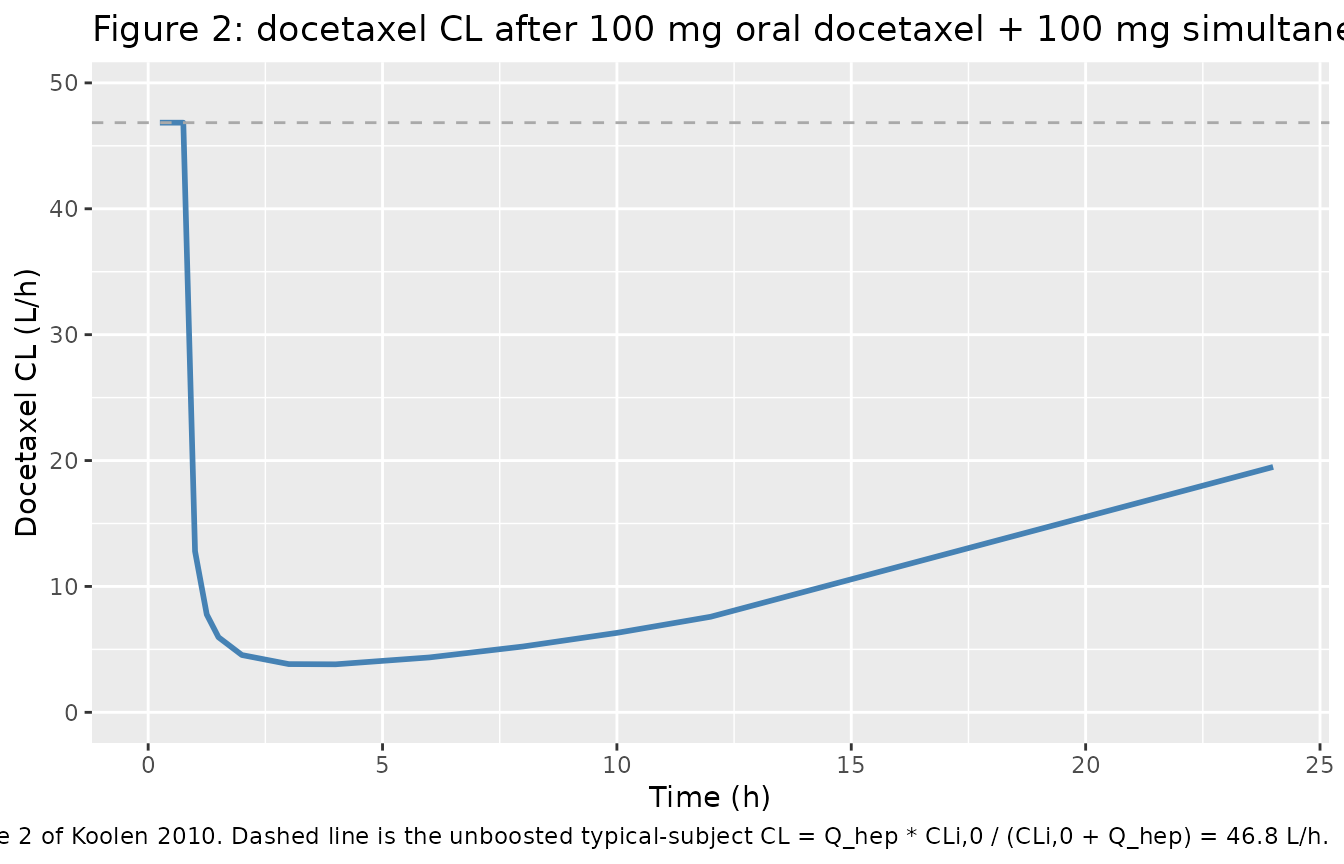
Visual predictive check of docetaxel concentrations
sim |>
  dplyr::filter(time >= 0, time <= 48) |>
  dplyr::group_by(treatment, time) |>
  dplyr::summarise(
    Q05 = quantile(Cc * 1000, 0.05, na.rm = TRUE),  # convert mg/L -> ng/mL
    Q50 = quantile(Cc * 1000, 0.50, na.rm = TRUE),
    Q95 = quantile(Cc * 1000, 0.95, na.rm = TRUE),
    .groups = "drop"
  ) |>
  ggplot(aes(time, Q50)) +
  geom_ribbon(aes(ymin = Q05, ymax = Q95), alpha = 0.25, fill = "steelblue") +
  geom_line(colour = "steelblue", linewidth = 0.8) +
  facet_wrap(~ treatment, ncol = 3) +
  scale_y_log10() +
  labs(x = "Time (h)", y = "Docetaxel Cc (ng/mL)",
       title = "Simulated 90% prediction band and median",
       caption = "Six of the ten RTV dose-and-timing regimens reported in Koolen 2010 Table 3.")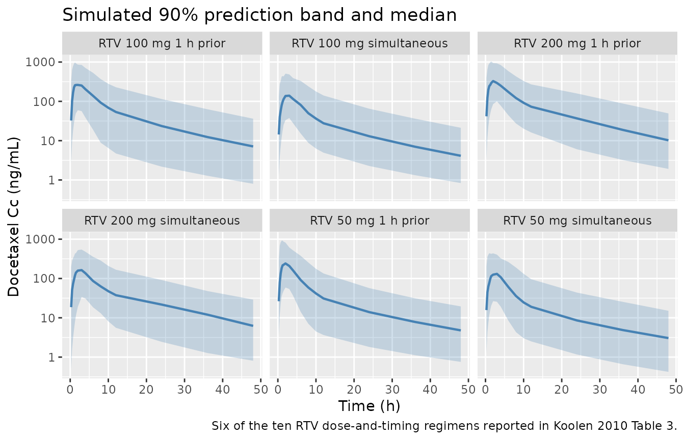
PKNCA validation
The chunk below derives AUC(0,inf) for each (id, treatment) using PKNCA and compares the geometric mean across subjects against the values printed in Koolen 2010 Table 3.
sim_nca <- sim |>
  dplyr::filter(!is.na(Cc)) |>
  dplyr::select(id, time, Cc, treatment) |>
  dplyr::mutate(Cc = Cc * 1000)  # convert mg/L -> ng/mL for the NCA output

# Guarantee a time = 0 row per (id, treatment); for extravascular pre-dose
# Cc = 0 is correct.
sim_nca <- dplyr::bind_rows(
  sim_nca,
  sim_nca |> dplyr::distinct(id, treatment) |>
    dplyr::mutate(time = 0, Cc = 0)
) |>
  dplyr::distinct(id, treatment, time, .keep_all = TRUE) |>
  dplyr::arrange(id, treatment, time)

conc_obj <- PKNCA::PKNCAconc(sim_nca, Cc ~ time | treatment + id,
                             concu = "ng/mL", timeu = "h")

# Doses: docetaxel dose only (NCA is for docetaxel; RTV is the perpetrator).
dose_df <- arms |>
  dplyr::filter(evid == 1, cmt == "depot") |>
  dplyr::select(id, time, amt, treatment)

dose_obj <- PKNCA::PKNCAdose(dose_df, amt ~ time | treatment + id,
                             doseu = "mg")

intervals <- data.frame(
  start       = 0,
  end         = Inf,
  cmax        = TRUE,
  tmax        = TRUE,
  aucinf.obs  = TRUE,
  half.life   = TRUE
)

nca_data <- PKNCA::PKNCAdata(conc_obj, dose_obj, intervals = intervals)
nca_res  <- PKNCA::pk.nca(nca_data)
Comparison against published Table 3
Koolen 2010 Table 3 reports geometric-mean AUC(0,inf) in mg/Lh units across 1000 simulated patients per regimen, with the 90% confidence interval in parentheses. The table below converts to ngh/mL (1 mg/Lh = 1000 ngh/mL) so both the simulated and the published columns use the same units used in the NCA output above.
geom_mean <- function(x) exp(mean(log(x[x > 0]), na.rm = TRUE))

sim_summary <- as.data.frame(nca_res$result) |>
  dplyr::filter(PPTESTCD == "aucinf.obs") |>
  dplyr::group_by(treatment) |>
  dplyr::summarise(sim_geomean = geom_mean(PPORRES), .groups = "drop")

# Published values from Koolen 2010 Table 3 (mg/L*h converted to ng*h/mL by
# multiplying by 1000).
published <- tibble::tribble(
  ~treatment,                       ~paper_geomean, ~paper_ci_lo, ~paper_ci_hi,
  "RTV 50 mg simultaneous",           1070,           1000,         1130,
  "RTV 100 mg simultaneous",          1360,           1280,         1450,
  "RTV 200 mg simultaneous",          1710,           1610,         2150,
  "RTV 50 mg 1 h prior",              1870,           1770,         1970,
  "RTV 100 mg 1 h prior",             2560,           2410,         2710,
  "RTV 200 mg 1 h prior",             3320,           3140,         3500
)

cmp <- dplyr::left_join(sim_summary, published, by = "treatment") |>
  dplyr::mutate(
    paper_geomean_pretty = sprintf("%.0f (%.0f, %.0f)",
                                   paper_geomean, paper_ci_lo, paper_ci_hi),
    pct_diff = 100 * (sim_geomean - paper_geomean) / paper_geomean
  ) |>
  dplyr::select(treatment, sim_geomean, paper_geomean_pretty, pct_diff)

cmp |>
  dplyr::rename(
    "Treatment"                                         = treatment,
    "Simulated AUC0-inf (ng*h/mL)"                      = sim_geomean,
    "Published AUC0-inf (ng*h/mL, geom. mean (90% CI))" = paper_geomean_pretty,
    "% diff (sim vs paper)"                             = pct_diff
  ) |>
  knitr::kable(
  digits = 1,
  caption = paste0("Geometric-mean AUC0-inf in 200 simulated patients per arm ",
                   "vs Koolen 2010 Table 3 (1000 simulated patients per arm; ",
                   "1 mg/L*h = 1000 ng*h/mL).")
)| Treatment | Simulated AUC0-inf (ng*h/mL) | Published AUC0-inf (ng*h/mL, geom. mean (90% CI)) | % diff (sim vs paper) |
|---|---|---|---|
| RTV 100 mg 1 h prior | 2584.9 | 2560 (2410, 2710) | 1.0 |
| RTV 100 mg simultaneous | 1530.9 | 1360 (1280, 1450) | 12.6 |
| RTV 200 mg 1 h prior | 3557.9 | 3320 (3140, 3500) | 7.2 |
| RTV 200 mg simultaneous | 1945.4 | 1710 (1610, 2150) | 13.8 |
| RTV 50 mg 1 h prior | 1936.6 | 1870 (1770, 1970) | 3.6 |
| RTV 50 mg simultaneous | 1159.2 | 1070 (1000, 1130) | 8.3 |
Assumptions and deviations
-
Embedded ritonavir PK is fixed at Kappelhoff 2005 typical
values. Koolen 2010 used MAP Bayesian posthoc per-subject
estimates from the Kappelhoff 2005 ritonavir popPK model (Koolen 2010
Methods, reference [8]). The packaged Koolen 2010 model embeds the
Kappelhoff 2005 typical values (CL/F = 10.5 L/h, V/F = 96.6 L, ka =
0.871 1/h, Tlag = 0.778 h) as
fixed()parameters with zero IIV so that the joint model is self-contained for simulation. Users who need per-subject ritonavir variability should simulate ritonavir concentrations frommodellib("Kappelhoff_2005_ritonavir")independently and supply the resulting profile as a time-varying input. -
Inter-occasion variability (IOV) is not propagated.
Koolen 2010 Table 2 reports IOV on CLi,0 (22%), MAT (52%), and F_RTV
(44%) – treatment courses in the source were three or more weeks apart
so per-cycle drift was identifiable. The packaged model carries only the
inter-individual etas. For simulation studies whose endpoint depends on
cycle-to-cycle variability, the IOV terms can be added on top by hand
using
rxode2’s occasion-block facilities. -
Elevated first-4-hour-after-oral proportional residual error
is not encoded. Koolen 2010 reports a 32% proportional RUV for
the final model plus a separately-estimated 63% proportional RUV for
docetaxel observations within the first 4 hours after oral
administration. Only the structural 32% term is propagated by
propSd. Users who want to overlay a piecewise RUV band on a VPC can post-process the simulatedCccolumn by multiplying the RUV envelope by 63 / 32 for observation records satisfyingROUTE_IV == 0andtad < 4 h. -
ROUTE_IVreference category is oral, not SC. The canonicalROUTE_IVininst/references/covariate-columns.mdhistorically used SC as the 0-reference category (Yu 2022, Zierhut 2008, Wang 2021, Fiedler-Kelly 2019). The Koolen 2010 paper pools IV and oral docetaxel cohorts; the packaged model usesROUTE_IV = 0for oral docetaxel andROUTE_IV = 1for IV docetaxel, with the V_central switch chosen accordingly. The ROUTE_IV register entry now documents this paper-specific reference category alongside the SC-reference precedent. - Correlation CL ~ V2 is applied to V_central_iv only. Koolen 2010 Table 2 reports a single 44.6% correlation between IIV on CL and IIV on V2 in the final model. The packaged model treats this as a correlation between the etas on CLi,0 and V_central_iv (the V2 that maps to the basic IV-only Bruno model carried forward into the final model); V_central_po carries an independent eta. The paper does not specify which V2 the correlation belongs to; the IV interpretation is the most natural carry-forward from the basic IV-only column of Table 2.
- Vignette uses 200 simulated subjects per arm, not 1000. Koolen 2010 Table 3 was generated from 1000 simulated subjects per arm; the validation vignette here uses 200 to keep render time under the 5 minute pkgdown gate. The geometric-mean point estimates remain a reasonable check; the paper’s 90% confidence intervals would tighten on larger N.