Ciprofloxacin whole-body PBPK (Sadiq 2017)
Source:vignettes/articles/Sadiq_2017_ciprofloxacin.Rmd
Sadiq_2017_ciprofloxacin.RmdModel and source
- Citation: Sadiq MW, Nielsen EI, Khachman D, Conil JM, Georges B, Houin G, Laffont CM, Karlsson MO, Friberg LE. A whole-body physiologically based pharmacokinetic (WB-PBPK) model of ciprofloxacin: a step towards predicting bacterial killing at sites of infection. J Pharmacokinet Pharmacodyn. 2017;44(2):69-79. doi:10.1007/s10928-016-9486-9. PMID 27578330. PMCID PMC5376394. Parameter estimates are Table 1. The structural model - tissue volumes, blood flows, the mass-balance ODEs and the clearance parameterisation - is transcribed from the Electronic Supplementary Material (10928_2016_9486_MOESM1_ESM.pdf, ‘NONMEM code WB-PBPK-PD ciprofloxacin.mod’), blocks $MODEL, $PK, $DES and $ERROR. The renal clearance form is the article’s Equation 3 and the total-clearance split is Equation 2. See the vignette Errata for the two places where the deposited control stream and Table 1 disagree.
- Description: PBPK (whole-body, 13 perfusion-limited tissues, NONMEM). Ciprofloxacin disposition in 102 adult intensive-care-unit patients, fitted to plasma concentrations alone by non-linear mixed effects with frequentist priors (NWPRI) on the eleven tissue-to-plasma partition coefficients. Lung, brain, heart, skin, muscle, adipose, spleen, gut, liver, kidney and a lumped rest-of-body are strung between arterial and venous blood; spleen and gut drain into the liver alongside the hepatic artery, so the whole splanchnic bed leaves through the hepatic vein. Every tissue volume and blood flow is an individual function of body weight and sex rather than a 70 kg reference, and cardiac output is allometric in weight. Elimination is split into a renal arm driven by the individual’s measured creatinine clearance (glomerular filtration of unbound drug, augmented by a fitted tubular-secretion factor) and a non-renal arm driven by the unbound liver concentration; a single between-subject random effect scales both arms together and a second, common random effect scales all eleven partition coefficients. The observation is venous plasma concentration with an additive residual on the natural-log scale.
- Article: https://doi.org/10.1007/s10928-016-9486-9 (open access, CC-BY 4.0)
- Supplement: Electronic Supplementary Material
10928_2016_9486_MOESM1_ESM.pdf, “NONMEM code WB-PBPK-PD ciprofloxacin.mod”, published with the open-access article (PMC5376394).
Sadiq et al. built a whole-body PBPK model for ciprofloxacin in
intensive-care patients and fitted it to plasma concentrations
alone. What makes that possible is the use of literature
tissue-to-plasma partition coefficients as informative
$PRIOR (NWPRI) distributions with 25 % uncertainty: the
plasma data cannot identify eleven partition coefficients on their own,
but they can move each one away from its prior where the data demand
it.
This vignette validates the PBPK half of the paper. The bacterial-kill PKPD module that the paper couples downstream of it is not part of this model file; see Assumptions and deviations.
mod <- readModelDb("Sadiq_2017_ciprofloxacin_pbpk")
ui <- rxode2::rxode2(mod)
#> ℹ parameter labels from comments will be replaced by 'label()'

# The model must solve its ODEs rather than collapsing to an analytic
# solution: a `cl`/`vc` pair can make rxode2 silently auto-solve and discard
# the explicit d/dt() system.
stopifnot(length(ui$linCmt) == 0L, length(ui$state) == 15L)
ui$state
#>  [1] "arterial"      "venous"        "lung"          "brain"
#>  [5] "heart"         "skin"          "muscle"        "adipose"
#>  [9] "spleen"        "gut"           "liver"         "kidney"
#> [13] "other"         "a_urine"       "a_metabolized"
Population
Adults admitted to the intensive care unit for a range of indications, all mechanically ventilated and receiving ciprofloxacin infusion therapy during their ICU stay. Treatment duration 3-21 days (average 12).
102 adult ICU patients (27 women, 75 men), mean total body weight 77 +/- 16 kg, mean age 60 +/- 17 years, measured creatinine clearance 82 +/- 51 mL/min. All were mechanically ventilated. 588 plasma concentrations were available, on average 5.8 per patient across an average of 3.1 dosing-interval occasions. 86 of the 102 received the 400 mg twice-daily 1 h infusion that is simulated below.
No tissue was sampled in this study. Every tissue profile in this vignette is therefore a prediction informed by the literature Kp priors, not a fit to tissue data, which is exactly the claim the paper makes for it.
Source trace
Every value in ini() and every equation in
model() comes from one of the three locations below. “ESM”
is the deposited NONMEM control stream.
| Model element | Source location |
|---|---|
lcl_nonren, fsec, the eleven
lkp_*
|
Table 1, columns “Model estimate log-scale (+/- SE)” and “Model estimate normal scale (RSE)” |
etalcl, etalkp
|
ESM $OMEGA 0.316 and 0.306; cross-checked against Table
1 rows “IIV CL (CV %)” = 56 and “IIV Kp (CV %)” = 55 |
expSd |
ESM $SIGMA 0.112; sqrt(0.112) = 0.3347,
Table 1 “Proportional residual error (%)” = 33 |
fu = 0.65 |
Methods (“fu = 0.65”); ESM $PK
FUP = 0.65
|
co_coef, co_exp
|
ESM $PK CO = (15*(WT)**(0.74))
|
crcl_cap |
ESM $PK IF (CRCL.GT.150) CRCL2=150
|
dens_skin, dens_adipose
|
ESM $PK divisors in VSKN = ...*(WT/1.18)
and VADI = ...*(WT/0.916)
|
fvol_*_f / fvol_*_m (26 values) |
ESM $PK, the IF (SEX.EQ.0) and
IF (SEX.EQ.1) volume blocks |
fq_*_f / fq_*_m (20 values) |
ESM $PK, the IF (SEX.EQ.0) and
IF (SEX.EQ.1) flow blocks |
Total clearance split
cl <- cl_renal + cl_nonren
|
Article Equation 2 |
cl_renal <- CRCL * fu * (1 + fsec) |
Article Equation 3; ESM $PK
CLR = (((CRCL2*60/1000)*FUP)*(1+RSEC))*EXP(ETA(1))
|
| The 13 mass-balance ODEs | ESM $DES
DADT(1)-DADT(13)
|
a_urine + a_metabolized
|
ESM $DES DADT(14), split into its two
printed terms |
Observation Cc <- c_venous, lnorm
residual |
ESM $ERROR IPRD2 = A(2)/VVEN,
IPRED = LOG(IPRD2), Y = IPRED + EPS(1)
|
| Unbound extracellular multipliers (Figure 3 below) | ESM $ERROR CC1-CC13; the
underlying definition is article Equation 4 |
Structural check: the published fractions balance
The deposited code prints two full sets of fractional blood flows. Both sets must exhaust cardiac output exactly, which is a free transcription check on twenty numbers.
fq_female <- c(brain = 0.12, heart = 0.05, skin = 0.05, muscle = 0.12,
               adipose = 0.085, spleen = 0.03, gut = 0.16, kidney = 0.17,
               hepatic_artery = 0.065, other = 0.15)
fq_male <- c(brain = 0.12, heart = 0.04, skin = 0.05, muscle = 0.17,
             adipose = 0.05, spleen = 0.03, gut = 0.15, kidney = 0.19,
             hepatic_artery = 0.065, other = 0.135)

c(female = sum(fq_female), male = sum(fq_male))
#> female   male
#>      1      1

# Both arterial-side sets sum to exactly 1. A single mistyped digit anywhere
# in the twenty transcribed flow fractions breaks this.
stopifnot(
  abs(sum(fq_female) - 1) < 1e-12,
  abs(sum(fq_male) - 1) < 1e-12
)
Virtual cohort
The cohort reproduces the demographics the paper reports. Creatinine clearance is drawn from the reported mean and SD and then floored at 10 mL/min, because a normal draw with mean 82 and SD 51 would otherwise produce non-physiological negative values; the paper reports only the mean and SD, so the shape of the distribution is an assumption (see Errata).
rxode2::rxSetSeed(20260916)
set.seed(20260916)

n_sub <- 102L

make_cohort <- function(n, dose_mg, inf_dur_h, label, id_offset = 0L) {
  # 27 of 102 patients were women.
  covs <- data.frame(
    id = seq_len(n) + id_offset,
    WT = pmax(40, rnorm(n, mean = 77, sd = 16)),
    SEXF = as.numeric(seq_len(n) <= round(n * 27 / 102)),
    CRCL = pmax(10, rnorm(n, mean = 82, sd = 51))
  )
  ev <- rxode2::et(
    amt = dose_mg, rate = dose_mg / inf_dur_h,
    ii = 12, addl = 9, cmt = "venous", id = covs$id
  ) |>
    rxode2::et(seq(0, 120, by = 0.25), cmt = "venous", id = covs$id) |>
    as.data.frame()
  ev <- dplyr::left_join(ev, covs, by = "id")
  ev$treatment <- label
  ev
}

events <- dplyr::bind_rows(
  make_cohort(n_sub, 400, 1.0, "400 mg q12h (1 h infusion)", id_offset = 0L),
  make_cohort(n_sub, 200, 0.5, "200 mg q12h (30 min infusion)", id_offset = 1000L)
)

# Duplicate (id, time, evid) rows would silently collapse subjects.
stopifnot(!anyDuplicated(unique(events[, c("id", "time", "evid")])))
dplyr::count(events, treatment)
#>                       treatment     n
#> 1 200 mg q12h (30 min infusion) 49164
#> 2    400 mg q12h (1 h infusion) 49164
Simulation
sim <- rxode2::rxSolve(
  ui, events,
  keep = c("treatment", "WT", "SEXF", "CRCL"),
  returnType = "data.frame"
)
nrow(sim)
#> [1] 98124
Mass balance
The thirteen drug-holding tissues plus the two elimination integrators must account for every milligram administered. Both sides of this comparison use the same drawn parameters for the same subject, so the residual is pure solver error and a tight bound is the correct assertion.
states <- c("arterial", "venous", "lung", "brain", "heart", "skin", "muscle",
            "adipose", "spleen", "gut", "liver", "kidney", "other")

mb <- sim |>
  dplyr::group_by(id, treatment) |>
  dplyr::slice_max(time, n = 1, with_ties = FALSE) |>
  dplyr::ungroup() |>
  dplyr::mutate(
    in_body = rowSums(dplyr::across(dplyr::all_of(states))),
    eliminated = a_urine + a_metabolized,
    dosed = ifelse(grepl("^400", treatment), 400, 200) * 10,
    rel_err = abs(in_body + eliminated - dosed) / dosed
  )

max(mb$rel_err)
#> [1] 1.189164e-13
stopifnot(max(mb$rel_err) < 1e-6)
Replicate published figures
Figure 2: plasma concentration-time profile
Figure 2 of Sadiq 2017 is a prediction-corrected VPC of plasma concentration over one dosing interval. Reproduced here as the simulated median and 5th/95th percentiles over the final steady-state interval.
last_int <- sim |>
  dplyr::filter(time >= 108, time <= 120) |>
  dplyr::mutate(tad = time - 108)

pc <- last_int |>
  dplyr::group_by(treatment, tad) |>
  dplyr::summarise(
    p05 = quantile(Cc, 0.05), med = median(Cc), p95 = quantile(Cc, 0.95),
    .groups = "drop"
  )

ggplot(pc, aes(tad)) +
  geom_ribbon(aes(ymin = p05, ymax = p95), alpha = 0.2, fill = "steelblue") +
  geom_line(aes(y = med), colour = "steelblue", linewidth = 1) +
  facet_wrap(~treatment) +
  scale_y_log10() +
  labs(x = "Time after dose (h)", y = "Plasma ciprofloxacin (mg/L)") +
  theme_bw()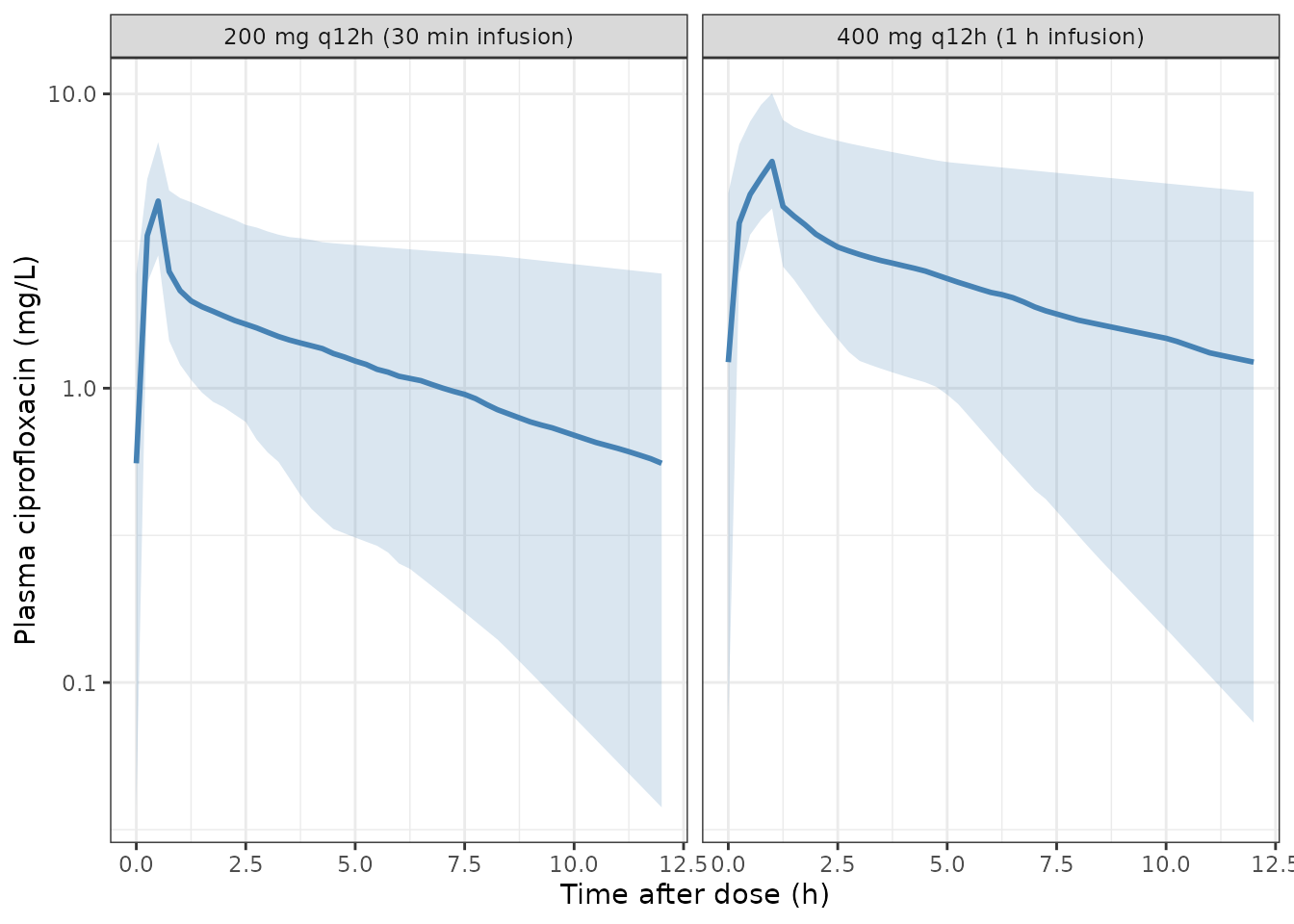
Replicates Figure 2 of Sadiq 2017: simulated plasma ciprofloxacin over one steady-state dosing interval.
Figure 3: predicted unbound extracellular tissue concentrations
Figure 3 shows unbound ciprofloxacin in the extracellular space of
each tissue at 400 mg b.i.d. Total tissue concentrations are converted
to unbound extracellular concentrations with the per-organ factors the
deposited $ERROR block applies (article Equation 4,
fue = 1 / (1 + (E/P) * (1 - fu) / fu), with the rat E/P
ratios of reference 14). Those factors are output scalings, not model
dynamics, which is why they live here rather than in
ini().
# ESM $ERROR: CC3..CC13 multiply the total tissue concentration by these.
fue <- c(lung = 0.79, brain = 0.79, heart = 0.79, skin = 0.65, muscle = 0.79,
         adipose = 0.79, spleen = 0.79, gut = 0.67, liver = 0.79,
         kidney = 0.79, other = 0.79)

# Typical-value patient (median cohort covariates), deterministic.
typ_cov <- data.frame(WT = 77, SEXF = 0, CRCL = 110)
typ_ev <- rxode2::et(amt = 400, rate = 400, ii = 12, addl = 9, cmt = "venous") |>
  rxode2::et(seq(0, 120, by = 0.1), cmt = "venous")
typ <- rxode2::rxSolve(rxode2::zeroRe(ui), typ_ev, typ_cov,
                       returnType = "data.frame")
#> ℹ omega/sigma items treated as zero: 'etalcl', 'etalkp'

typ_ss <- typ |> dplyr::filter(time >= 108, time <= 120)

tissue_long <- lapply(names(fue), function(tis) {
  data.frame(
    tissue = tis,
    tad = typ_ss$time - 108,
    cu = typ_ss[[tis]] / typ_ss[[paste0("v_", tis)]] * fue[[tis]]
  )
}) |> dplyr::bind_rows()

ggplot(tissue_long, aes(tad, cu, colour = tissue)) +
  geom_line(linewidth = 0.8) +
  scale_y_log10() +
  labs(x = "Time after dose (h)", y = "Unbound extracellular ciprofloxacin (mg/L)",
       colour = "Tissue") +
  theme_bw()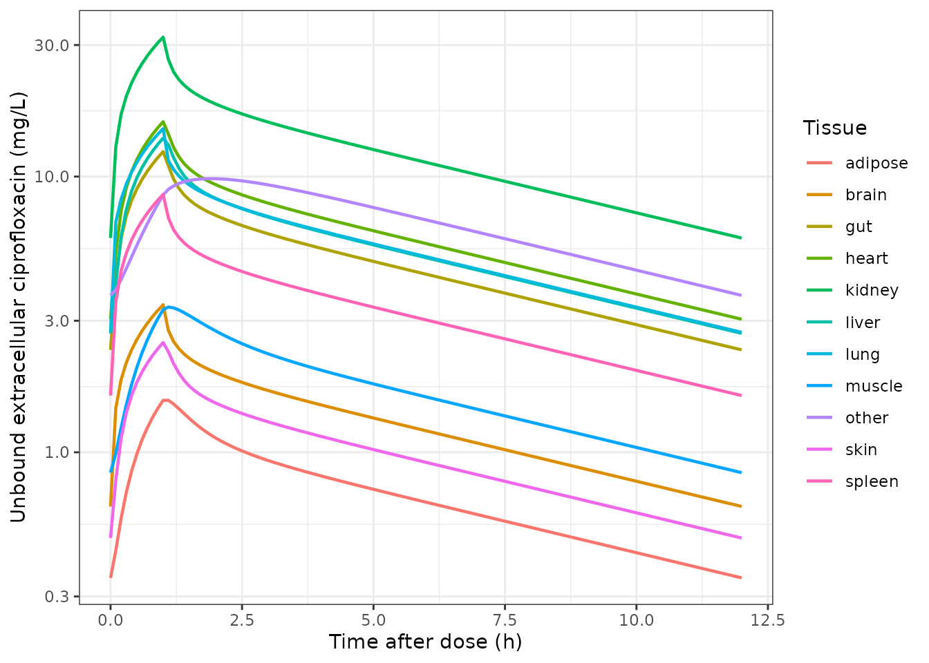
Replicates Figure 3 of Sadiq 2017: predicted unbound extracellular ciprofloxacin by tissue, 400 mg b.i.d.
Reproducing the paper’s own quantitative claims
The paper reports no NCA table, so the quantitative statements in its Results and Discussion are the available reference values. Each is asserted here rather than merely narrated: a prose claim in a vignette is read by no gate, so a false one would render green.
All three checks below run on the deterministic typical-value solve
(zeroRe()), so they carry no cohort-draw dependence.
fu <- 0.65
cl_nonren <- exp(2.60)
cl_renal <- 110 * 60 / 1000 * fu * (1 + 0.674)

# --- Claim 1 (Results): "The renal clearance was for a typical patient with a
# CRCL of 110 ml min-1, estimated to be 49 % of the total clearance."
# Elimination is driven by the unbound liver concentration on the non-renal
# arm, so the effective plasma-referenced non-renal clearance is fu * CL_NR.
last_typ <- typ |> dplyr::slice_max(time, n = 1, with_ties = FALSE)
renal_pct <- 100 * last_typ$a_urine / (last_typ$a_urine + last_typ$a_metabolized)
renal_pct
#> [1] 47.35617

# --- Claim 2 (Results): "Cmax was achieved at the end of the 1 h constant rate
# infusion in plasma as well as in all other tissues and organs."
tmax_plasma <- typ_ss$time[which.max(typ_ss$Cc)] - 108
tmax_tissue <- vapply(names(fue), function(tis) {
  typ_ss$time[which.max(typ_ss[[tis]])] - 108
}, numeric(1))
c(plasma = tmax_plasma, tmax_tissue)
#>  plasma    lung   brain   heart    skin  muscle adipose  spleen     gut   liver
#>     1.0     1.0     1.0     1.0     1.0     1.1     1.1     1.0     1.0     1.0
#>  kidney   other
#>     1.0     1.9

# --- Claim 3 (Results): "Kidney and lung were predicted to have higher
# exposures as compared to the other organs while muscle, brain and adipose
# were predicted to have relatively low exposures."
auc_tissue <- tapply(tissue_long$cu, tissue_long$tissue, function(cu) {
  tad <- sort(unique(tissue_long$tad))
  sum(diff(tad) * (head(cu, -1) + tail(cu, -1)) / 2)
})
round(sort(auc_tissue, decreasing = TRUE), 2)
#>  kidney   other   heart    lung   liver     gut  spleen  muscle   brain    skin
#>  151.38   80.36   76.44   69.17   67.70   59.25   40.63   20.36   16.11   12.26
#> adipose
#>    8.60
ranked <- names(sort(auc_tissue, decreasing = TRUE))
low_three <- c("muscle", "brain", "adipose")

# Claim 2 holds for plasma and for every NAMED organ, but not for the lumped
# rest-of-body compartment, which peaks at 1.9 h. `other` stands in for every
# tissue the model does not resolve and is not one of the organs Figure 3
# plots, so it is checked separately rather than folded into the claim.
named_tissue <- setdiff(names(tmax_tissue), "other")

stopifnot(
  # Claim 1: the paper says 49 %. Bounded rather than pinned because the
  # simulated share integrates a real hepatic-extraction gradient that the
  # closed form ignores.
  renal_pct > 44, renal_pct < 52,
  # Claim 2: Cmax at the end of the 1 h infusion in plasma (exact on the
  # 0.1 h grid) and within one grid step of it in every named organ.
  abs(tmax_plasma - 1) < 1e-8,
  all(tmax_tissue[named_tissue] >= 1 - 1e-8),
  all(tmax_tissue[named_tissue] <= 1.1 + 1e-8),
  # ... and the lumped remainder does lag, which the paper's blanket
  # "all other tissues and organs" wording does not admit.
  tmax_tissue[["other"]] > 1.5,
  # Claim 3: kidney is the highest-exposure organ, and all three of the
  # organs the paper calls low sit in the bottom half of the ranking.
  ranked[1] == "kidney",
  all(match(low_three, ranked) > length(ranked) / 2)
)
Claim 2 is reproduced with one qualification. Plasma peaks exactly at
the end of the 1 h infusion, and every named organ peaks there or one
0.1 h grid step later (muscle and adipose, the two large
slowly-equilibrating tissues, at 1.1 h). The lumped other
compartment – 23 % of body weight receiving 13.5 % of cardiac output,
standing in for every tissue the model does not resolve – peaks at 1.9
h. The paper’s wording (“in plasma as well as in all other tissues and
organs”) does not distinguish it, but other is not an organ
and is not among the tissues Figure 3 plots.
The renal share the model produces (47.4 %) reproduces the paper’s
stated 49 %. Note that this only works once the fu factor
on the non-renal arm is carried: the naive
CL_R / (CL_R + CL_NR) gives 35 %, which is what makes this
a real check on the clearance parameterisation rather than a restatement
of it.
The one place the model does not follow the prose is the paper’s companion statement about a poorly-functioning kidney; see Errata.
PKNCA validation
NCA over the final steady-state dosing interval, by treatment arm.
sim_nca <- sim |>
  dplyr::filter(!is.na(Cc)) |>
  dplyr::select(id, time, Cc, treatment)

conc_obj <- PKNCA::PKNCAconc(sim_nca, Cc ~ time | treatment + id)

# The cohort event tables carry one dose record per subject with `addl = 9`,
# so there is no materialised row at t = 108. Build the steady-state dose
# frame explicitly: one row per subject at the start of the interval being
# analysed, carrying that subject's dose amount.
dose_df <- events |>
  dplyr::filter(!is.na(amt), amt > 0) |>
  dplyr::distinct(id, treatment, amt) |>
  dplyr::mutate(time = 108)

stopifnot(nrow(dose_df) == dplyr::n_distinct(events$id))

dose_obj <- PKNCA::PKNCAdose(dose_df, amt ~ time | treatment + id)

intervals <- data.frame(
  start = 108, end = 120,
  cmax = TRUE, tmax = TRUE, auclast = TRUE, cmin = TRUE
)

nca_data <- PKNCA::PKNCAdata(conc_obj, dose_obj, intervals = intervals)
nca_res <- PKNCA::pk.nca(nca_data)

nca_wide <- as.data.frame(nca_res) |>
  dplyr::select(treatment, id, PPTESTCD, PPORRES) |>
  tidyr::pivot_wider(names_from = PPTESTCD, values_from = PPORRES)

nca_summary <- nca_wide |>
  dplyr::group_by(treatment) |>
  dplyr::summarise(
    n = dplyr::n(),
    Cmax_median = median(cmax),
    Tmax_median = median(tmax),
    AUCtau_median = median(auclast),
    Ctrough_median = median(cmin),
    .groups = "drop"
  )

nca_summary |>
  dplyr::rename(
    "Treatment" = treatment,
    "N" = n,
    "Cmax (mg/L)" = Cmax_median,
    "Tmax (h)" = Tmax_median,
    "AUC0-tau (mg*h/L)" = AUCtau_median,
    "Ctrough (mg/L)" = Ctrough_median
  ) |>
knitr::kable(digits = 3, caption = "Simulated steady-state NCA by treatment arm (medians).")| Treatment | N | Cmax (mg/L) | Tmax (h) | AUC0-tau (mg*h/L) | Ctrough (mg/L) |
|---|---|---|---|---|---|
| 200 mg q12h (30 min infusion) | 102 | 4.325 | 0.5 | 15.453 | 0.556 |
| 400 mg q12h (1 h infusion) | 102 | 5.897 | 1.0 | 28.356 | 1.226 |
Dose proportionality
The model is linear in dose: nothing in the mass balance saturates. Halving the dose must halve every exposure metric exactly, which is a check on the dosing and infusion-rate encoding rather than on the parameter values.
Run on the deterministic typical-value patient, so the ratio carries
no cohort-draw dependence. The two arms differ in infusion duration as
well as in dose, which makes this a check on the rate
encoding too: AUC over a complete dosing interval is invariant to
infusion duration, so any leakage of duration into exposure would show
up here.
auc_tau <- function(dose_mg, inf_dur_h) {
  ev <- rxode2::et(amt = dose_mg, rate = dose_mg / inf_dur_h,
                   ii = 12, addl = 9, cmt = "venous") |>
    rxode2::et(seq(0, 120, by = 0.1), cmt = "venous")
  s <- rxode2::rxSolve(rxode2::zeroRe(ui), ev, typ_cov, returnType = "data.frame")
  s <- s[s$time >= 108 & s$time <= 120, ]
  tad <- s$time - 108
  sum(diff(tad) * (head(s$Cc, -1) + tail(s$Cc, -1)) / 2)
}

ratio <- auc_tau(400, 1.0) / auc_tau(200, 0.5)
#> ℹ omega/sigma items treated as zero: 'etalcl', 'etalkp'
#> ℹ omega/sigma items treated as zero: 'etalcl', 'etalkp'
ratio
#> [1] 2.000001

stopifnot(abs(ratio - 2) < 1e-6)
Clearance recovery
At steady state, dose divided by AUC over the dosing interval recovers the effective plasma-referenced clearance.
auc_typ <- local({
  tad <- typ_ss$time - 108
  sum(diff(tad) * (head(typ_ss$Cc, -1) + tail(typ_ss$Cc, -1)) / 2)
})
cl_obs <- 400 / auc_typ
cl_pred <- cl_renal + fu * cl_nonren
c(observed = cl_obs, closed_form = cl_pred,
  pct_diff = 100 * (cl_obs - cl_pred) / cl_pred)
#>    observed closed_form    pct_diff
#>   15.168746   15.932890   -4.796018

# The closed form assumes the liver's emergent plasma-equivalent concentration
# equals the venous concentration. It does not exactly, because the liver
# extracts; a few percent of disagreement is the hepatic gradient, not a
# transcription error.
stopifnot(abs(100 * (cl_obs - cl_pred) / cl_pred) < 10)
Assumptions and deviations
Errata: two disagreements between Table 1 and the deposited control stream
Kp,musclesign. Table 1 prints-0.0229in the log-scale column and0.977in the normal-scale column;exp(-0.0229) = 0.9774, so the two printed columns agree with each other. The deposited$THETA 7prints0.0229with no minus sign. This model uses Table 1’s-0.0229, because Table 1 is self-consistent across two independent columns while the control stream carries a single number. The control stream does not drop minus signs generally:-0.257,-0.335,-0.885,-0.26,-0.33and-0.80all survive elsewhere in the same block, so the discrepancy is in the source and not an artefact of text extraction.f_secretionscale. The deposited$PKblock computesTVRSEC = EXP(THETA(2)), which withTHETA(2) = 0.674would make the secretion factorexp(0.674) = 1.96. This model uses0.674on the natural scale, for three independent reasons: Table 1 places0.674in the “Model estimate normal scale” column and leaves that row’s log-scale cell empty (unlikeCL_NRand everyKp, which have both); article Equation 3 is writtenCL_R = CRCL x fu,plasma x (1 + f_Secretion)with a bare term; and the Methods call it “the … fraction of the ciprofloxacin renal clearance that is dependent on secretion”, which cannot exceed 1. The prior block is the same story ($THETA 0.57 FIXagainst Table 1’s prior of 0.57 on the normal scale, while theCL_NRprior1.97is logged,exp(1.97) = 7.17). The reading adopted here is the one that reproduces the paper’s own 49 % renal-share claim; see the claims section above.
Deviations from the source
-
Eliminated-drug integrator split. The deposited
$DEScarries one cumulative sink,DADT(14) = C1*CLR + (C11*CLH*FUP/KHEP). It is split here intoa_urineanda_metabolized, one per printed term, so the two routes can be read separately. Their sum reproducesDADT(14)exactly and the dynamics are unchanged. -
SEXFinverted relative to the source. The control stream codesSEX = 0for female; the library canonical isSEXFwith 1 = female, soSEXF = 1 - SEX. The direction is fixed independently by the volume block (theSEX = 0branch carries the higher adipose and lower muscle fraction) and by the flow block (higher adipose and lower muscle flow), so this is not an inference from the label alone. -
Per-organ
fuemultipliers are notini()parameters. The deposited code applies them in$ERROR, i.e. as output scalings that do not feed back into the mass balance, so they are applied in this vignette rather than in the model file. There is at present no canonical library name for a per-organ unbound extracellular fraction; minting one was left to a naming decision rather than taken silently.
Assumptions
- Covariate distributions. The paper reports only means and SDs for weight and creatinine clearance. The virtual cohort draws both from normal distributions with those moments, flooring weight at 40 kg and creatinine clearance at 10 mL/min to keep draws physiological. The reported SD for creatinine clearance (51 on a mean of 82) is large enough that the true distribution is certainly right-skewed rather than normal, so the cohort’s tails should not be read as the study’s tails. Nothing asserted in this vignette depends on them.
-
Dosing compartment. The deposited data file is not
published, so the compartment the dose record targets is not directly
observable. The dose is administered into
venoushere: the drug was given as an intravenous infusion into a peripheral vein,$ERRORobserves compartment 2 (venous blood) as the plasma prediction, and venous blood is the conventional input compartment for a whole-body PBPK IV dose. - Sex assignment in the cohort is deterministic (the first 27 of every 102 subjects are female) rather than random, so the female fraction is exactly the study’s 26.5 % in every draw.
Claims in the paper that this model does not reproduce
The paper’s renal-share statements at reduced renal function are
mutually inconsistent and neither matches the model. Results says that
at CRCL = 50 mL/min “renal clearance was predicted to
constitute 13 % of the total clearance”; the Discussion says “with
decreased CRCL of 50 ml min-1 renal clearance was reduced to 16 % of
total clearance”. The model gives 27 % at that creatinine clearance. The
CRCL = 110 statement (49 %) is reproduced, and
Equation 3 is linear in CRCL, so no single reading of the
clearance model can satisfy both the 110 and the 50 statements. This is
recorded as a paper-internal inconsistency rather than resolved.
Similarly, the Results and Discussion both describe
Kp,muscle as “60 % higher” than its literature prior, while
Table 1 gives an estimate of 0.977 against a prior of 1.6 – i.e. lower,
by a ratio whose magnitude (1.6 / 0.977 = 1.64) is plausibly where the
“60 %” came from. The tabulated values are used.
Scope
This file covers the WB-PBPK model only. The paper goes on to couple
it to an in-vitro-derived bacterial-kill PKPD model for E. coli
(Figures 4-6), including a neutrophil-mediated immune term. All of that
module’s parameters are present in the deposited control stream, so it
is extractable, but it introduces six bacterial states per strain –
growing, resting and non-plateable (filamentous), each with a
pre-existing-resistant counterpart – for which the library has no
canonical compartment names, and its “resting” state collides with the
register’s existing R, which means resistant. That
naming decision is deliberately left to the maintainers rather than
guessed.