Methotrexate (Ruhs 2012) • nlmixr2lib

Model and source

Citation: Ruhs H, Becker A, Drescher A, Panetta JC, Pui CH, Relling MV, Jaehde U. Population PK/PD Model of Homocysteine Concentrations after High-Dose Methotrexate Treatment in Patients with Acute Lymphoblastic Leukemia. PLoS ONE. 2012;7(9):e46015. doi:[10.1371/journal.pone.0046015](https://doi.org/10.1371/journal.pone.0046015).
Article (open access): https://doi.org/10.1371/journal.pone.0046015
Drug: methotrexate (high-dose IV); homocysteine as PD biomarker.

The integrated PK/PD model couples a two-compartment population PK model for methotrexate (MTX) to a single-compartment indirect response model for homocysteine (HCY). MTX inhibits the HCY elimination rate constant kout via an inverse Emax function (Emax fixed to 1); the typical HCY baseline depends linearly on age (Ruhs 2012 Table 2 / Figure 2).

Population

The model was developed using data from 494 children with newly diagnosed acute lymphoblastic leukemia enrolled in the Total Therapy XV study at St. Jude Children’s Research Hospital (Memphis TN) and Cook Children’s Medical Center (Fort Worth TX). The cohort was split 2:1 into an index dataset (331 patients, 6722 MTX concentrations + 2567 HCY concentrations) and an external evaluation dataset (163 patients). Children received 4-hour or 24-hour MTX infusions during the window phase (1000 mg/m^2) followed by HDMTX consolidation cycles individualized to target an MTX steady-state plasma concentration of 33 uM (LR; ~2500 mg/m^2 median) or 65 uM (SHR; ~5000 mg/m^2 median). The same metadata is exposed programmatically via readModelDb("Ruhs_2012_methotrexate")$population.

mod_fn <- readModelDb("Ruhs_2012_methotrexate")
mod    <- rxode2::rxode(mod_fn)
#> ℹ parameter labels from comments will be replaced by 'label()'
str(mod$population)
#> List of 20
#>  $ species       : chr "human"
#>  $ n_subjects    : int 494
#>  $ n_index       : int 331
#>  $ n_evaluation  : int 163
#>  $ n_centres     : int 2
#>  $ n_mtx_obs     : int 6722
#>  $ n_hcy_obs     : int 2567
#>  $ age_range     : chr "1.03-18.85 years"
#>  $ age_median    : chr "5.42 years (index dataset)"
#>  $ weight_range  : chr "7.8-160.1 kg"
#>  $ weight_median : chr "22.0 kg (index dataset)"
#>  $ bsa_range     : chr "0.40-2.97 m^2"
#>  $ bsa_median    : chr "0.83 m^2"
#>  $ creat_range   : chr "0.1-1.2 mg/dL"
#>  $ sex_female_pct: num 42.9
#>  $ race_ethnicity: logi NA
#>  $ disease_state : chr "Newly diagnosed acute lymphoblastic leukemia (ALL); low-risk (LR) and standard/high-risk (SHR) subgroups strati"| __truncated__
#>  $ dose_range    : chr "Window therapy: 1000 mg/m^2 over 4 h (1 g/m^2) or over 24 h (200 mg/m^2 IV bolus followed by 800 mg/m^2 over 24"| __truncated__
#>  $ regions       : chr "USA (St. Jude Children's Research Hospital, Memphis TN; Cook Children's Medical Center, Fort Worth TX)"
#>  $ notes         : chr "Demographics from Ruhs 2012 Table 1. The PK model was developed on the index dataset (331 patients) and externa"| __truncated__
str(mod$covariateData)
#> List of 4
#>  $ BSA      :List of 6
#>   ..$ description       : chr "Body surface area"
#>   ..$ units             : chr "m^2"
#>   ..$ type              : chr "continuous"
#>   ..$ reference_category: NULL
#>   ..$ notes             : chr "Linear multiplicative scaling on CL, V1, Q, V2 (theta values in Table 2 are reported per m^2 BSA; the implicit "| __truncated__
#>   ..$ source_name       : chr "BSA"
#>  $ CREAT    :List of 6
#>   ..$ description       : chr "Measured serum creatinine"
#>   ..$ units             : chr "mg/dL"
#>   ..$ type              : chr "continuous"
#>   ..$ reference_category: NULL
#>   ..$ notes             : chr "Patient's measured serum creatinine (Ruhs 2012 Table 1: median 0.4 mg/dL, range 0.1-1.2). Enters the model only"| __truncated__
#>   ..$ source_name       : chr "CCR"
#>  $ CREAT_REF:List of 6
#>   ..$ description       : chr "Age- and gender-adjusted reference serum creatinine"
#>   ..$ units             : chr "mg/dL"
#>   ..$ type              : chr "continuous"
#>   ..$ reference_category: NULL
#>   ..$ notes             : chr "Externally-computed expected normal SCR for the individual (denoted CCR,adj in Ruhs 2012). The paper cites its "| __truncated__
#>   ..$ source_name       : chr "CCR,adj"
#>  $ AGE      :List of 6
#>   ..$ description       : chr "Age at study entry"
#>   ..$ units             : chr "years"
#>   ..$ type              : chr "continuous"
#>   ..$ reference_category: NULL
#>   ..$ notes             : chr "Time-fixed at study entry. Enters the model only as a linear additive effect on the typical HCY baseline: HCYBL"| __truncated__
#>   ..$ source_name       : chr "AGE"

Source trace

The per-parameter origin is recorded as an inline comment next to each ini() entry in inst/modeldb/specificDrugs/Ruhs_2012_methotrexate.R. The table below collects them in one place for review. All parameter values come from Ruhs 2012 Table 2 unless otherwise noted.

Equation / parameter	Value	Source location
`lcl` – MTX CL (per m^2 BSA)	log(6.68) L/h/m^2	Table 2 theta_CL = 6.68
`lvc` – MTX V1 (per m^2 BSA)	log(18.6) L/m^2	Table 2 theta_V1 = 18.6
`lq` – MTX Q (per m^2 BSA)	log(0.161) L/h/m^2	Table 2 theta_Q = 0.161
`lvp` – MTX V2 (per m^2 BSA)	log(3.09) L/m^2	Table 2 theta_V2 = 3.09
`e_creat_cl`	0.314	Table 2 theta_CR; Eq. 1 power on (CCR,adj / CCR)
`lhcybl` – HCY baseline at age 0 y	log(4.88) uM	Table 2 theta_BL = 4.88 (linear-age intercept)
`lkout` – HCY kout	log(0.027) 1/h	Table 2 theta_kout = 0.027
`lec50` – MTX EC50 for HCY inhibition	log(0.648) uM	Table 2 theta_EC50 = 0.648
`emax` – max fractional inhibition (FIXED)	1	Table 2 theta_Emax (fixed); Methods Eq. 3
`e_age_hcybl` – linear age effect on HCY baseline	0.116 uM/year	Table 2 theta_BL,AGE = 0.116
`etalcl` IIV variance	0.02089	Table 2 CL IIV 14.53% CV; omega^2 = log(1 + CV^2)
`etalvc` IIV variance	0.03199	Table 2 V1 IIV 18.03% CV
`etalq` IIV variance	0.12584	Table 2 Q IIV 36.61% CV
`etalhcybl` IIV variance	0.03528	Table 2 HCYBL IIV 18.95% CV
`etalkout` IIV variance	0.10472	Table 2 kout IIV 33.23% CV
`etalec50` IIV variance	0.25285	Table 2 EC50 IIV 53.63% CV
`propSd` – MTX prop. residual SD	0.235	Table 2 PK exponential error (small-sigma equivalent)
`addSd_HCY` – HCY add. residual SD	0.911 uM	Table 2 PD additive error
`propSd_HCY` – HCY prop. residual SD	0.165	Table 2 PD exponential error (small-sigma equivalent)
`CL = theta_CL * BSA * (CREAT_REF / CREAT)^theta_CR`	n/a	Equation 1
`d/dt(central), d/dt(peripheral1)`	n/a	Figure 2 (PK scheme)
Steady-state HCYBL = kin / kout	n/a	Equation 2
`d/dt(effect) = kin - kout * (1 - Emax * Cc/(EC50+Cc)) * effect`	n/a	Equation 3 (inverse Emax inhibition)

The conversion from MTX amount (mg) to MTX concentration (uM) uses MW = 454.44 g/mol baked into the model (MW_MTX); EC50 and HCY are reported by the paper in uM and the model preserves those units.

Virtual cohort

The original observed data are not publicly available. The simulations below use virtual populations whose covariate distributions approximate the published trial demographics (Ruhs 2012 Table 1). For the renal-function factor, CREAT_REF is set equal to CREAT so the factor evaluates to 1 (no adjustment) – the paper’s reference [23] formula for the age- and gender-adjusted reference SCR is not reproduced in the main text. See the Assumptions and deviations section below.

set.seed(20120925L)  # Ruhs 2012 publication date

# A typical pediatric ALL patient: age 5 years, BSA ~0.83 m^2 (Table 1
# medians). MTX doses follow the published Cpss-targeted regimen:
# LR target 33 uM, SHR target 65 uM, both as a 24-hour IV infusion with
# the loading-then-maintenance split simplified to a uniform 24-h infusion.
n_per_arm <- 200L

make_arm <- function(n, dose_mg_per_m2, treatment, id_offset = 0L) {
  ids <- id_offset + seq_len(n)
  bsa     <- pmax(0.4, pmin(2.97, rlnorm(n, log(0.83),   0.40)))   # m^2
  age     <- pmax(1.0, pmin(18.9, rlnorm(n, log(5.42),   0.55)))   # years
  creat   <- pmax(0.1, pmin(1.2,  rlnorm(n, log(0.4),    0.30)))   # mg/dL
  total_dose_mg <- dose_mg_per_m2 * bsa
  infusion_h    <- 24
  rate_mg_per_h <- total_dose_mg / infusion_h

  cov_df <- data.frame(id = ids, BSA = bsa, AGE = age,
                       CREAT = creat, CREAT_REF = creat)
  dose_rows <- data.frame(
    id   = ids,
    time = 0,
    amt  = total_dose_mg,
    rate = rate_mg_per_h,
    evid = 1L,
    cmt  = "central"
  ) |> merge(cov_df, by = "id", sort = FALSE)

  # One cmt = "Cc" observation per (id, time); the rxSolve output
  # carries both Cc and HCY columns at every observation time.
  obs_times <- c(seq(0, 24, by = 0.5), seq(25, 96, by = 1))
  obs_rows <- expand.grid(id = ids, time = obs_times) |>
    transform(amt = 0, rate = 0, evid = 0L, cmt = "Cc") |>
    merge(cov_df, by = "id", sort = FALSE)

  rows <- rbind(dose_rows, obs_rows)
  rows <- rows[order(rows$id, rows$time, rows$evid), ]
  rows$treatment <- treatment
  rows
}

events <- bind_rows(
  make_arm(n_per_arm, dose_mg_per_m2 = 2500, treatment = "LR (target Cpss 33 uM)",
           id_offset = 0L),
  make_arm(n_per_arm, dose_mg_per_m2 = 5000, treatment = "SHR (target Cpss 65 uM)",
           id_offset = n_per_arm)
)
stopifnot(!anyDuplicated(unique(events[, c("id", "time", "evid")])))

Simulation

sim <- rxode2::rxSolve(
  mod_fn, events = events,
  keep = c("treatment", "BSA", "AGE", "CREAT", "CREAT_REF"),
  returnType = "data.frame"
)
#> ℹ parameter labels from comments will be replaced by 'label()'

Replicate Figure 3 (MTX VPC)

Reproduce the visual predictive check of MTX concentration vs. time, by treatment arm. Ruhs 2012 Figure 3 panels A and B show the 90% prediction interval of 10000 simulations for dose levels of 2500 +/- 20 mg/m^2 and 5000 +/- 20 mg/m^2.

mtx_vpc <- sim |>
  filter(time > 0) |>
  group_by(time, treatment) |>
  summarise(
    Q05 = quantile(Cc, 0.05, na.rm = TRUE),
    Q50 = quantile(Cc, 0.50, na.rm = TRUE),
    Q95 = quantile(Cc, 0.95, na.rm = TRUE),
    .groups = "drop"
  )

ggplot(mtx_vpc, aes(time, Q50, group = treatment, colour = treatment, fill = treatment)) +
  geom_ribbon(aes(ymin = Q05, ymax = Q95), alpha = 0.20, colour = NA) +
  geom_line(linewidth = 0.9) +
  scale_y_log10() +
  labs(x = "Time after start of MTX infusion (h)",
       y = "MTX concentration (uM)",
       title = "Figure 3 -- MTX VPC by HDMTX dose level",
       caption = "Replicates Ruhs 2012 Figure 3 (panels A LR / B SHR). 200 virtual patients per arm.") +
  theme_minimal()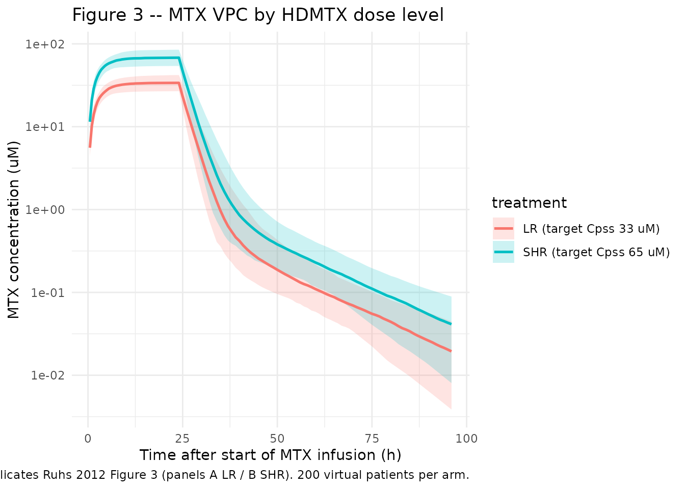

Replicate Figure 4 (HCY change from baseline)

Ruhs 2012 Figure 4 shows the VPC for HCY change from baseline, stratified by LR / SHR risk group. The vertical scale is HCY minus the individual baseline, so a positive deviation indicates MTX-driven accumulation.

sim_hcy <- sim |>
  group_by(id) |>
  mutate(HCY_baseline = HCY[time == 0][1],
         HCY_delta    = HCY - HCY_baseline) |>
  ungroup() |>
  filter(time > 0)

hcy_vpc <- sim_hcy |>
  group_by(time, treatment) |>
  summarise(
    Q05 = quantile(HCY_delta, 0.05, na.rm = TRUE),
    Q50 = quantile(HCY_delta, 0.50, na.rm = TRUE),
    Q95 = quantile(HCY_delta, 0.95, na.rm = TRUE),
    .groups = "drop"
  )

ggplot(hcy_vpc, aes(time, Q50, group = treatment, colour = treatment, fill = treatment)) +
  geom_ribbon(aes(ymin = Q05, ymax = Q95), alpha = 0.20, colour = NA) +
  geom_line(linewidth = 0.9) +
  labs(x = "Time after start of MTX infusion (h)",
       y = "HCY change from baseline (uM)",
       title = "Figure 4 -- HCY VPC by HDMTX dose level",
       caption = "Replicates Ruhs 2012 Figure 4 (panels A LR / B SHR). 200 virtual patients per arm.") +
  theme_minimal()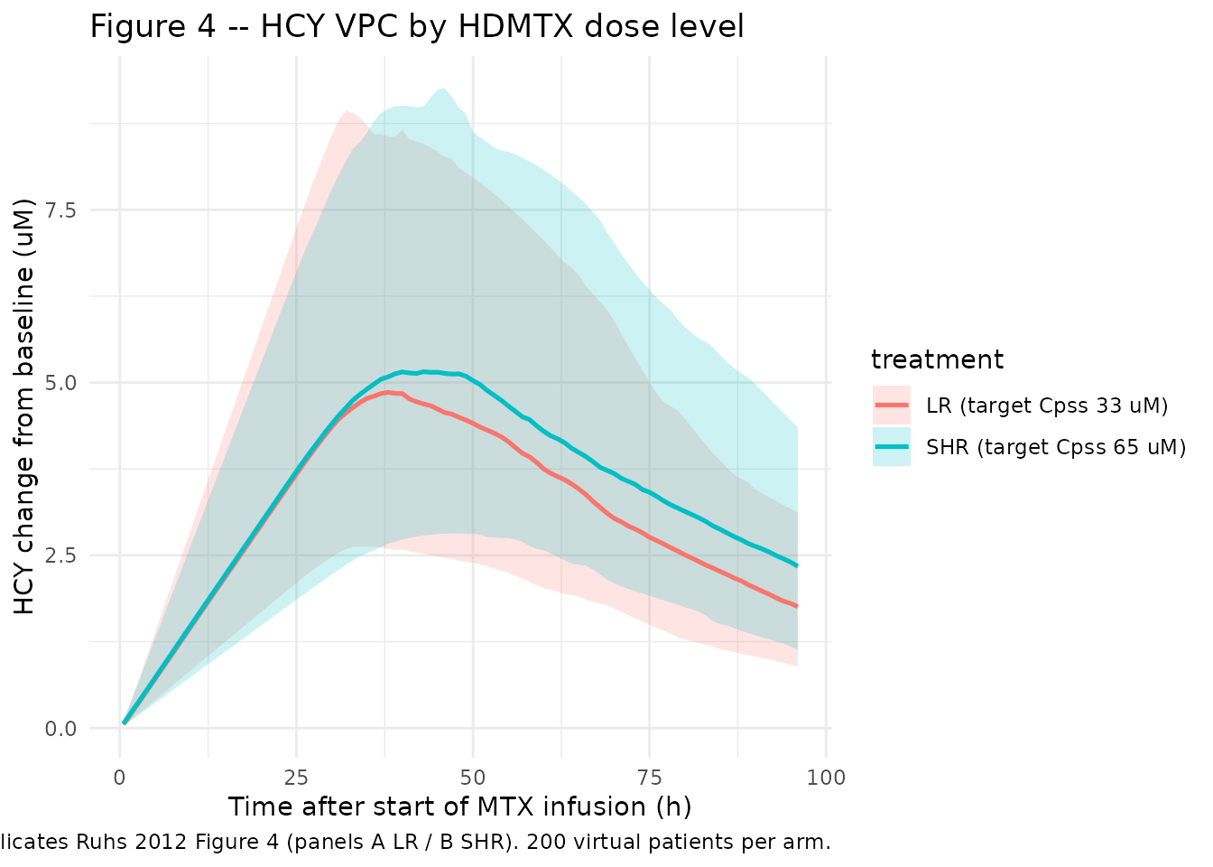

PKNCA validation (MTX)

PKNCA computes Cmax, Tmax, AUC, and half-life on the MTX concentration profile for each subject within each treatment arm.

sim_nca <- sim |>
  filter(!is.na(Cc)) |>
  select(id, time, Cc, treatment)

conc_obj <- PKNCA::PKNCAconc(sim_nca, Cc ~ time | treatment + id)

dose_df <- events |>
  filter(evid == 1) |>
  select(id, time, amt, treatment)

dose_obj <- PKNCA::PKNCAdose(dose_df, amt ~ time | treatment + id)

intervals <- data.frame(
  start       = 0,
  end         = 96,
  cmax        = TRUE,
  tmax        = TRUE,
  aucinf.obs  = TRUE,
  half.life   = TRUE
)

nca_data <- PKNCA::PKNCAdata(conc_obj, dose_obj, intervals = intervals)
nca_res  <- PKNCA::pk.nca(nca_data)

nca_summary <- summary(nca_res)
knitr::kable(nca_summary, caption = "Simulated MTX NCA parameters by HDMTX dose group.")

Simulated MTX NCA parameters by HDMTX dose group.
start	end	treatment	N	cmax	tmax	half.life	aucinf.obs
0	96	LR (target Cpss 33 uM)	200	33.8 [14.9]	24.0 [24.0, 24.0]	14.8 [4.98]	819 [15.1]
0	96	SHR (target Cpss 65 uM)	200	68.3 [13.9]	24.0 [24.0, 24.0]	15.1 [5.37]	1650 [14.1]

Comparison against published HCY summaries

Ruhs 2012 Results (page 2) reports median HCY Cmax and AUC over baseline for each risk subgroup. The simulation below approximates the without-folinate scenario from the paper’s Effect of Folinate Rescue section (median tmax of HCY reached at 15 hours after the end of MTX infusion in the LR group; 19.3 hours in the SHR group without folinate).

hcy_summary <- sim_hcy |>
  group_by(id, treatment) |>
  summarise(
    HCY_max_delta   = max(HCY_delta, na.rm = TRUE),
    HCY_max_total   = max(HCY,       na.rm = TRUE),
    HCY_auc_overBL  = sum((pmax(0, HCY_delta[-1]) + pmax(0, HCY_delta[-length(HCY_delta)])) / 2 *
                          diff(time)),
    .groups = "drop"
  ) |>
  group_by(treatment) |>
  summarise(
    median_HCY_max   = median(HCY_max_total),
    p05_HCY_max      = quantile(HCY_max_total, 0.05),
    p95_HCY_max      = quantile(HCY_max_total, 0.95),
    median_HCY_AUC   = median(HCY_auc_overBL),
    p05_HCY_AUC      = quantile(HCY_auc_overBL, 0.05),
    p95_HCY_AUC      = quantile(HCY_auc_overBL, 0.95),
    .groups = "drop"
  )

knitr::kable(hcy_summary, caption = "Simulated HCY Cmax (uM, total concentration) and AUC over baseline (uM*h) by HDMTX dose group; 90% prediction interval (5th / 95th percentile).")

Simulated HCY Cmax (uM, total concentration) and AUC over baseline (uM*h) by HDMTX dose group; 90% prediction interval (5th / 95th percentile).
treatment	median_HCY_max	p05_HCY_max	p95_HCY_max	median_HCY_AUC	p05_HCY_AUC	p95_HCY_AUC
LR (target Cpss 33 uM)	10.76256	7.129635	17.15573	301.7009	169.5669	524.7031
SHR (target Cpss 65 uM)	10.87453	7.490848	16.46455	333.5324	202.6401	571.0168

The published medians from Ruhs 2012 (without folinate):

Subgroup	Cmax HCY (uM)	90% PI Cmax	AUC over baseline (uM*h)	90% PI AUC
LR	9.37	5.73-15.77	1615	951-2765
SHR	10.70	6.37-17.84	2107	1207-3510

Differences from the simulation reflect cohort-composition choices made for this vignette (200 vs 1000 patients; CREAT_REF set equal to CREAT; simplified 24-hour infusion vs the paper’s load-and-maintain split). The structural levels and dose-ordering (SHR > LR for both Cmax and AUC) reproduce the qualitative claims in Ruhs 2012 Discussion.

Assumptions and deviations

MTX mg dose to uM concentration conversion. The model accepts MTX dosing in mg into the central compartment and converts the central compartment amount to a uM observation via (central / vc) * 1000 / MW_MTX (MW_MTX = 454.44 g/mol), so that EC50 and HCY remain in the published uM units. checkModelConventions() emits a dimensional-incompatibility WARN between units$dosing (mg) and units$concentration (umol/L); this is expected and is preserved by design, matching the pattern in Ahn_2014_parathyroidHormone.R.
NONMEM exponential error converted to nlmixr2 proportional error. Ruhs 2012 Table 2 reports an MTX exponential residual SD = 0.235 (PK) and a combined HCY additive 0.911 uM + exponential 0.165 (PD). The model encodes these as Cc ~ prop(propSd) and HCY ~ prop(propSd_HCY) + add(addSd_HCY) with the proportional SD set equal to the NONMEM exponential SD. This is the standard small-sigma equivalent of NONMEM’s exponential error model (Y = F * exp(EPS) ~= F * (1 + EPS) for small EPS); at sigma = 0.235 the implied %CV differs by ~3% between the two parameterisations, and at sigma = 0.165 the difference is ~1.4%, both negligible for simulation. The combined add() + lnorm() form is not natively supported as a simulation-time residual error model in nlmixr2 (only as additive + proportional), so the small-sigma equivalent is used in the packaged model.
CREAT_REF set equal to CREAT. The paper’s renal-function factor on CL uses an age- and gender-adjusted reference SCR (CCR,adj) computed per the cited reference [23] (a maturation-dependent Schwartz-derived formula). The main paper text does not give the explicit formula. In this vignette CREAT_REF is set equal to CREAT so the factor evaluates to 1 and the population-typical CL applies. Users with patient-level data should compute CREAT_REF externally per the paper’s reference [23] before passing the data to rxSolve(). See inst/references/covariate-columns.md (entry CREAT_REF) for the canonical convention.
Linear BSA scaling. Ruhs 2012 reports PK parameters per m^2 BSA without fitting an exponent on BSA, i.e. the implicit BSA exponent is 1. The model file applies * BSA to CL, V1, Q, V2 directly. For paediatric patients with BSA much smaller than 1 m^2 the linear scaling assumption is conservative relative to a fractional-power allometric scaling.
IOV not encoded. The paper estimated interoccasion variability (IOV) on CL (17.15% CV) and HCYBL (23.83% CV) across the window phase and the four consolidation HDMTX administrations. nlmixr2 does not have a first-class IOV construct; the packaged model encodes only the between-subject IIV. Users wanting to simulate occasion-aware data can add an occasion-indexed eta on lcl and lhcybl following the standard nlmixr2 IOV pattern; the variances to use are log(1 + 0.1715^2) = 0.02906 and log(1 + 0.2383^2) = 0.05541.
Linear age effect on HCY baseline. The model uses HCYBL_tv = theta_BL + theta_BL,AGE * AGE with log-normal IIV applied to the typical value. The paper does not explicitly state whether IIV is on the additive sum or only on the intercept; the typical-value formulation follows the standard NONMEM popPK convention for additive-then-multiplicative parameterization.
Inverse Emax interpretation. Ruhs 2012 describes Emax as ‘the remaining fraction to which kout will be reduced at the maximal effect of MTX.’ The numerics in the Discussion section (‘HCY elimination rate (kout) was reduced to 1.93 and 0.99% of the baseline kout, respectively’ at the LR and SHR Cpss targets) match the conventional inverse-Emax form kout' = kout * (1 - Emax * Cc / (EC50 + Cc)) with Emax = 1, which is the form encoded in the model file. The wording in the paper is somewhat ambiguous on the precise interpretation of Emax; the math is unambiguous given the reported residual-kout fractions.
No folinate rescue. The model represents the unrescued PK/PD coupling only. The paper’s folinate simulations were performed by simplifying Equation 3 (removing the MTX inhibition term during the rescue window), which is straightforward to add as a post-hoc time-conditional in the user’s own model() extension if needed; the unrescued model is the structural reference and is encoded here.
Race / ethnicity not reported. Ruhs 2012 Table 1 does not break down race/ethnicity, so the cohort here does not encode race indicators.