Vixarelimab (Tang 2026)
Source:vignettes/articles/Tang_2026_vixarelimab.Rmd
Tang_2026_vixarelimab.RmdModel and source
ui <- rxode2::rxode(readModelDb("Tang_2026_vixarelimab"))
#> ℹ parameter labels from comments will be replaced by 'label()'- Citation: Tang F, Dang S, Arjomandi A, Pan L, Hsu J, Kshirsagar S, Kassir N. Population Pharmacokinetic Analysis of Vixarelimab in Healthy Volunteers and Patients With Chronic Pruritic Conditions. CPT Pharmacometrics Syst Pharmacol. 2026;15(3):e70230. doi:10.1002/psp4.70230
- Description: Two-compartment target-mediated drug-disposition (TMDD) model with a quasi-steady-state (QSS) approximation for subcutaneous and intravenous vixarelimab (anti-OSMR-beta monoclonal antibody) in healthy volunteers and patients with chronic pruritic conditions, with first-order absorption, logit-scale bioavailability and power body-weight effects on CL, Vc and Vp (Tang 2026, Table 3)
- Article: https://doi.org/10.1002/psp4.70230 (open access)
- Supporting Information (Tables S1-S5, Figures S1-S6 and the
full NONMEM control stream for the final model):
psp470230-sup-0001-Supinfo.docx, published with the open-access article (PMC13140993).
Vixarelimab (KPL-716) is a fully human monoclonal antibody against oncostatin M receptor beta (OSMR-beta). Because it binds both membrane-bound and soluble OSMR, its disposition is target-mediated: apparent clearance is high at low concentrations and saturates as the dose increases. Tang and colleagues described this with a two-compartment target-mediated drug disposition (TMDD) model using the quasi-steady-state (QSS) approximation, plus a first-order subcutaneous absorption depot.
Population
The analysis pooled 4032 serum concentrations collected; 3328 quantifiable post-dose samples used for model fitting (Section 3.1) from 274 participants across 3 studies: the Phase 1 first-in-human study KPL-716-C001 (Parts 1, 3 and 4) and the Phase 2 studies KPL-716-C201 (NCT03816891, Phases 2a and 2b) and KPL-716-C202 (NCT03858634).
Per Table 2 of the source, the participants had a median (range) age of 52 years (18-79 years) and weight of 82 kg (48-158 kg); 58% were female and 68% were White. Fourteen percent were healthy volunteers and 86% had a chronic pruritic skin disorder (atopic dermatitis, prurigo nodularis, or one of five other chronic pruritic diseases). 50 of 274 participants (18%) had at least one positive post-baseline anti-drug-antibody result (Table 2).
Dose levels spanned IV single doses 0.3, 1.5, 5, 7.5, 10 and 20 mg/kg; SC single doses 1.5 mg/kg and 360 mg; SC multiple doses 360 mg QW, 720 mg SC loading followed by 360 mg QW, and 120/360/540 mg Q4W (Table 1).
The same information is available programmatically via
readModelDb("Tang_2026_vixarelimab")()$population.
Model structure
The authors’ model (Section 2.4, Equations 2-6, and the Supporting
Information $DES block) is reproduced exactly. Writing
Ctot = Ac/Vc for the total drug concentration in the
central compartment and Rtot for the total (free plus
drug-bound) receptor concentration:
dAsc /dt  = -Ka * Asc                                                    (Eq 2)
dAc  /dt  =  Ka * Asc - (Kel + Kpt) * Cfree * Vc + Ktp * Ap
             - Rtot * Kint * Cfree * Vc / (Kss + Cfree)                  (Eq 3)
dAp  /dt  =  Kpt * Cfree * Vc - Ktp * Ap                                 (Eq 4)
dRtot/dt  =  Ksyn - Kdeg * Rtot - (Kint - Kdeg) * Rtot * Cfree/(Kss+Cfree)(Eq 5)

Cfree     =  0.5 * [ (Ctot - Rtot - Kss)
                     + sqrt( (Ctot - Rtot - Kss)^2 + 4 * Kss * Ctot ) ]  (Eq 6)
with Kel = CL/Vc, Kpt = Q/Vc,
Ktp = Q/Vp, Ksyn = Kdeg * R0 and the receptor
compartment started at its baseline, Rtot(0) = R0.
Two details are load-bearing and are easy to get wrong:
-
The model is molar.
R0andKssare estimated in nM, and Equation 6 subtracts them from the drug concentration, so the drug states carry nmol andtotal_targetcarries nM. The packaged model accepts doses in mg and reportsCcin ug/mL, converting with a molecular weight (see Assumptions and deviations). -
The observation is the FREE concentration, not the
total. The assay does not detect vixarelimab when both binding
sites are occupied (Section 2.2), and the authors’
$ERRORblock predictsLOG(CFREE). The packaged model therefore setsCc <- cfree * mw / 1e6.
Source trace
Every ini() value carries an in-file comment naming its
source location in
inst/modeldb/specificDrugs/Tang_2026_vixarelimab.R. They
are collected here.
| Equation / parameter | Value | Source location |
|---|---|---|
lvc (Vc) |
3.04 L | Table 3, “Central volume of distribution, Vc (L)” |
lcl (CL) |
0.00649 L/h | Table 3, “Clearance, CL (L/h)” |
lq (Q) |
0.0207 L/h | Table 3, “Inter-compartmental clearance, Q (L/h)” |
lvp (Vp) |
1.74 L | Table 3, “Peripheral volume of distribution, Vp (L)” |
lka (Ka) |
0.0126 1/h | Table 3, “Absorption rate constant, Ka (h-1)” |
logitfdepot (F1) |
56.6% | Table 3, “Subcutaneous bioavailability, F (%)”; logit scale per
$PK
|
lrbase (R0) |
1.84 nM | Table 3, “Baseline receptor level, R0 (nM)” |
lkdeg (Kdeg) |
0.097 1/h | Table 3, “Receptor degradation rate constant, Kdeg (h-1)” |
lkss (Kss) |
0.0296 nM | Table 3, “Quasi steady-state rate constant, Kss (nM)” |
lkint (Kint) |
0.000141 1/h | Table 3, “Complex elimination rate constant Kint (h-1)” |
e_wt_cl |
0.943 | Table 3, “Weight on CL” |
e_wt_vc |
0.762 | Table 3, “Weight on Vc” |
e_wt_vp |
0.646 | Table 3, “Weight on Vp” |
| WT centring constant | 81.7 kg | Supporting Information $PK:
CLWT = ((WT/81.7)**THETA(11))
|
etalvc |
CV 18.1% | Table 3, “Between subject variability for Vc (CV%)” |
etalcl |
CV 24.9% | Table 3, “Between subject variability for CL (CV%)” |
etalq |
CV 91.6% | Table 3, “Between subject variability for Q (CV%)” |
etalrbase |
CV 42.8% | Table 3, “Between subject variability for R0 (CV%)” |
etalka |
CV 51.1% | Table 3, “Between subject variability for Ka (CV%)” |
etalogitfdepot |
CV 42.1% | Table 3, “Between subject variability for F1 (CV%)” |
etalvp |
fixed 0 | Section 3.2; Supporting Information $OMEGA,
0 FIX ; ETA_VP
|
expSd |
CV 19.6% | Table 3, “Log-additive residual variability (CV%)” |
| Eq 2-5 (ODEs) | n/a | Section 2.4, Equations 2-5; Supporting Information
$DES
|
| Eq 6 (QSS root) | n/a | Section 2.4, Equation 6; Supporting Information
$DES
|
Rtot(0) = R0 |
n/a | Supporting Information $PK:
A_0(3) = BLR
|
Cc = Cfree |
n/a | Section 2.2; Supporting Information $ERROR:
IPRED = LOG(CFREE + DEL)
|
Table 3 reports interindividual and residual variability as
CV% = sqrt(exp(omega^2) - 1) * 100% (footnotes b and c), so
the packaged variances are
omega^2 = log(1 + (CV/100)^2).
knitr::kable(
  ui$iniDf |>
    dplyr::filter(is.na(neta1)) |>
    dplyr::select(name, est, label) |>
    dplyr::rename("Parameter" = name, "Estimate" = est, "Label" = label),
  digits = 6, caption = "Fixed effects as packaged."
)| Parameter | Estimate | Label |
|---|---|---|
| lvc | 1.111858 | Central volume of distribution (L) |
| lcl | -5.037493 | Linear (non-specific) clearance (L/h) |
| lq | -3.877622 | Inter-compartmental clearance (L/h) |
| lvp | 0.553885 | Peripheral volume of distribution (L) |
| lka | -4.374058 | First-order subcutaneous absorption rate constant (1/h) |
| logitfdepot | 0.265550 | Subcutaneous bioavailability on the logit scale (logit(F1), unitless) |
| lrbase | 0.609766 | Baseline total target (OSMR-beta) concentration (nM) |
| lkdeg | -2.333044 | Target degradation rate constant (1/h) |
| lkss | -3.519981 | Quasi-steady-state constant for drug-target binding (nM) |
| lkint | -8.866751 | Drug-target complex internalisation rate constant (1/h) |
| e_wt_cl | 0.943000 | Power exponent of WT/81.7 on CL (unitless) |
| e_wt_vc | 0.762000 | Power exponent of WT/81.7 on Vc (unitless) |
| e_wt_vp | 0.646000 | Power exponent of WT/81.7 on Vp (unitless) |
| expSd | 0.194156 | Log-scale, log-additive, residual standard deviation (unitless) |
Virtual cohort
The original observed data are not public. The cohorts below draw body weights from a log-normal distribution matched to Table 2 (median 82 kg, truncated to the observed 48-158 kg range), which is the only covariate in the final model.
draw_wt <- function(n) pmin(pmax(stats::rlnorm(n, log(82), 0.21), 48), 158)

# Build one cohort as a self-contained event table. Observation rows point at
# the ODE state `central`; rxode2 returns the algebraic observable `Cc` (and the
# other model variables) as columns at those rows.
make_arm <- function(n, dose_mg_per_kg = NULL, dose_mg = NULL, route = c("iv", "sc"),
                     ii = 0, addl_doses = 0, obs_times, label, id_offset = 0L) {
  route <- match.arg(route)
  subj <- tibble::tibble(id = id_offset + seq_len(n), WT = draw_wt(n), arm = label)
  dose_amt <- if (is.null(dose_mg)) dose_mg_per_kg * subj$WT else dose_mg
  dosing <- subj |>
    dplyr::mutate(amt = dose_amt, evid = 1L,
                  cmt = if (route == "iv") "central" else "depot") |>
    tidyr::crossing(dose_index = seq_len(addl_doses + 1L)) |>
    dplyr::mutate(time = (dose_index - 1L) * ii) |>
    dplyr::select(-dose_index)
  obs <- subj |>
    tidyr::crossing(time = obs_times) |>
    dplyr::mutate(amt = NA_real_, evid = 0L, cmt = "central")
  dplyr::bind_rows(dosing, obs) |> dplyr::arrange(id, time, dplyr::desc(evid))
}

WEEK <- 168  # hours
LLOQ <- 0.4  # ug/mL, the ELISA lower limit of quantification for C001 Parts 1 and 3 (Section 2.2)
Figure 1: single-dose profiles and dose-dependent nonlinearity
Figure 1 of the source shows observed serum concentrations after single IV and SC doses in KPL-716-C001 Parts 1 (atopic dermatitis) and 3 (healthy volunteers). The hallmark of target-mediated disposition is visible as a steep terminal drop at low doses that flattens as the dose rises.
iv_doses <- c(0.3, 1.5, 5, 7.5, 10, 20)
obs_grid <- c(seq(0, 24, by = 2), seq(36, WEEK, by = 12), seq(WEEK + 24, WEEK * 12, by = 24))

sd_arms <- dplyr::bind_rows(lapply(seq_along(iv_doses), function(i) {
  make_arm(200, dose_mg_per_kg = iv_doses[i], route = "iv", obs_times = obs_grid,
           label = paste0(iv_doses[i], " mg/kg IV"), id_offset = (i - 1L) * 200L)
}))
sd_arms$arm <- factor(sd_arms$arm, levels = paste0(iv_doses, " mg/kg IV"))

sd_sim <- rxode2::rxSolve(ui, sd_arms, keep = c("WT", "arm"), returnType = "data.frame") |>
  dplyr::filter(!is.na(Cc)) |>
  dplyr::mutate(Cc = pmax(Cc, 0))
#> ℹ omega/sigma items treated as zero: 'etalvp'

sd_sim |>
  dplyr::group_by(arm, time) |>
  dplyr::summarise(Q05 = quantile(Cc, 0.05), Q50 = median(Cc), Q95 = quantile(Cc, 0.95),
                   .groups = "drop") |>
  dplyr::filter(Q50 > LLOQ / 10) |>
  ggplot(aes(time / WEEK, Q50, colour = arm, fill = arm)) +
  geom_ribbon(aes(ymin = Q05, ymax = Q95), alpha = 0.15, colour = NA) +
  geom_line(linewidth = 0.7) +
  geom_hline(yintercept = LLOQ, linetype = "dashed") +
  scale_y_log10() +
  coord_cartesian(xlim = c(0, 12), ylim = c(0.2, 1000)) +
  labs(x = "Time after dose (weeks)", y = "Vixarelimab serum concentration (ug/mL)",
       colour = "Treatment", fill = "Treatment",
       title = "Single IV doses: median and 5th-95th percentile",
       caption = "Replicates Figure 1 of Tang 2026. Dashed line = 0.4 ug/mL LLOQ.")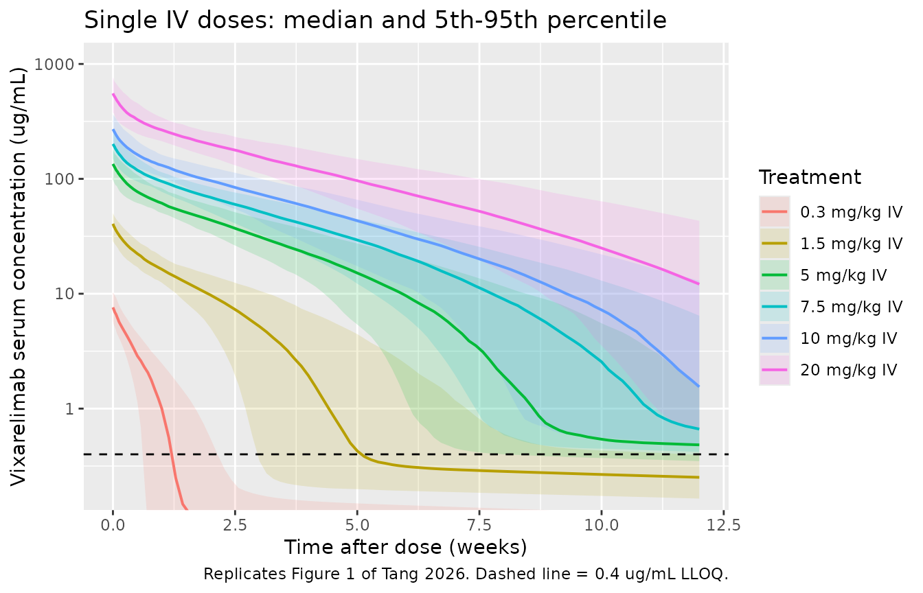
The simulated envelopes span the same concentration range as the observations in Figure 1 (roughly 1-1000 ug/mL over 0-12 weeks), and reproduce the characteristic convex-down terminal descent at the lower doses.
PKNCA: saturation of the nonlinear clearance (Figure S1)
Section 3.1 states that “dose-normalized vixarelimab concentration-time profiles following IV single doses in healthy volunteers overlapped in the initial weeks after dosing at doses >= 5 mg/kg, at which point systemic PK approached linearity, indicating saturation of the nonlinear clearance (Figure S1).”
Non-compartmental analysis is performed with PKNCA.
Following the source’s own handling, concentrations below the 0.4 ug/mL
LLOQ are removed (Figure 1 caption) and the window is capped at the 12
weeks shown in Figure 1.
The NCA runs on the typical-value profile of each
dose level rather than on the 200-participant cohorts plotted above.
rxSetSeed() fixes rxode2’s RNG per solver thread and not
across thread counts, so a cohort median carries a sampling error of
roughly 2% that varies from machine to machine – and the adjacent
dose-normalised AUC values here differ by as little as 4%. Running the
NCA on the deterministic typical-value profile removes that noise
entirely and lets the assertions below be exact instead of loosened to
survive it.
ui_typ <- rxode2::zeroRe(ui)

tv_arms <- dplyr::bind_rows(lapply(seq_along(iv_doses), function(i) {
  meta <- tibble::tibble(id = i, WT = 82,
                         arm = factor(paste0(iv_doses[i], " mg/kg IV"),
                                      levels = paste0(iv_doses, " mg/kg IV")))
  dplyr::bind_rows(
    dplyr::mutate(meta, time = 0, amt = iv_doses[i] * 82, evid = 1L, cmt = "central"),
    tidyr::crossing(meta, time = obs_grid) |>
      dplyr::mutate(amt = NA_real_, evid = 0L, cmt = "central")
  ) |>
    dplyr::arrange(time, dplyr::desc(evid))
}))

tv_sim <- suppressWarnings(
  rxode2::rxSolve(ui_typ, tv_arms, keep = c("WT", "arm"), returnType = "data.frame")
) |>
  dplyr::filter(!is.na(Cc)) |>
  dplyr::mutate(Cc = pmax(Cc, 0))
#> ℹ omega/sigma items treated as zero: 'etalvc', 'etalcl', 'etalq', 'etalrbase', 'etalka', 'etalogitfdepot', 'etalvp'

nca_conc <- tv_sim |>
  dplyr::filter(time <= WEEK * 12) |>
  dplyr::filter(Cc >= LLOQ | time == 0) |>
  dplyr::select(id, time, Cc, arm)

# Time-zero anchor for AUC (an IV bolus is observed at t = 0, so this is a no-op
# guard rather than an imputation).
nca_conc <- dplyr::bind_rows(
  nca_conc,
  nca_conc |> dplyr::distinct(id, arm) |> dplyr::mutate(time = 0, Cc = 0)
) |>
  dplyr::distinct(id, arm, time, .keep_all = TRUE) |>
  dplyr::arrange(id, arm, time)

stopifnot(nrow(nca_conc) > 0, all(nca_conc$Cc >= 0))

conc_obj <- PKNCA::PKNCAconc(as.data.frame(nca_conc), Cc ~ time | arm + id)
dose_obj <- PKNCA::PKNCAdose(
  as.data.frame(dplyr::select(dplyr::filter(tv_arms, evid == 1), id, time, amt, arm)),
  amt ~ time | arm + id
)

intervals <- data.frame(start = 0, end = Inf,
                        cmax = TRUE, tmax = TRUE, aucinf.obs = TRUE, cl.obs = TRUE)
nca_res <- suppressWarnings(
  PKNCA::pk.nca(PKNCA::PKNCAdata(conc_obj, dose_obj, intervals = intervals))
)
nca_tab <- as.data.frame(nca_res$result) |>
  dplyr::filter(PPTESTCD %in% c("cmax", "tmax", "aucinf.obs", "cl.obs")) |>
  dplyr::select(arm, PPTESTCD, value = PPORRES) |>
  tidyr::pivot_wider(names_from = PPTESTCD, values_from = value) |>
  dplyr::mutate(
    dose_mg_per_kg = as.numeric(sub(" .*", "", as.character(arm))),
    auc_dose_norm  = aucinf.obs / dose_mg_per_kg
  ) |>
  dplyr::arrange(dose_mg_per_kg) |>
  dplyr::mutate(auc_dn_rel = auc_dose_norm / auc_dose_norm[dose_mg_per_kg == 5])

knitr::kable(
  nca_tab |>
    dplyr::select(arm, cmax, tmax, aucinf.obs, cl.obs, auc_dose_norm, auc_dn_rel) |>
    dplyr::rename("Treatment" = arm, "Cmax (ug/mL)" = cmax, "Tmax (h)" = tmax,
                  "AUC0-inf (ug*h/mL)" = aucinf.obs, "CL (L/h)" = cl.obs,
                  "AUC/dose ((ug*h/mL)/(mg/kg))" = auc_dose_norm,
                  "AUC/dose vs 5 mg/kg" = auc_dn_rel),
  digits = c(0, 1, 1, 0, 5, 0, 3),
  caption = paste(
    "NCA parameters of the typical 82 kg participant at each dose level.",
    "PKNCA's cl.obs is dose/AUC in the supplied units, i.e. L/h here."
  )
)| Treatment | Cmax (ug/mL) | Tmax (h) | AUC0-inf (ug*h/mL) | CL (L/h) | AUC/dose ((ug*h/mL)/(mg/kg)) | AUC/dose vs 5 mg/kg |
|---|---|---|---|---|---|---|
| 0.3 mg/kg IV | 7.8 | 0 | 620 | 0.03969 | 2066 | 0.222 |
| 1.5 mg/kg IV | 40.1 | 0 | 8572 | 0.01435 | 5715 | 0.615 |
| 5 mg/kg IV | 134.2 | 0 | 46448 | 0.00883 | 9290 | 1.000 |
| 7.5 mg/kg IV | 201.5 | 0 | 72528 | 0.00848 | 9670 | 1.041 |
| 10 mg/kg IV | 268.7 | 0 | 100980 | 0.00812 | 10098 | 1.087 |
| 20 mg/kg IV | 537.7 | 0 | 222165 | 0.00738 | 11108 | 1.196 |
Three published statements are testable from this table.
dn <- setNames(nca_tab$auc_dose_norm, nca_tab$dose_mg_per_kg)
cl <- setNames(nca_tab$cl.obs, nca_tab$dose_mg_per_kg)
cl_linear <- exp(ui$theta[["lcl"]])

# These quantities come from deterministic typical-value solves, not from a
# sampled cohort, so they are reproducible on any machine and thread count and
# the bounds can be exact. Observed values are recorded alongside each bound.
stopifnot(
  # (1) Strongly nonlinear below 5 mg/kg: dose-normalised AUC rises >3-fold
  #     between 0.3 and 5 mg/kg. Observed 4.50.
  dn[["5"]] / dn[["0.3"]] > 3,
  # (2) Approaching linearity at and above 5 mg/kg: dose-normalised AUC varies
  #     by less than 25% across the 4-fold range from 5 to 20 mg/kg.
  #     Observed 1.196.
  dn[["20"]] / dn[["5"]] < 1.25,
  # (3) Apparent CL falls monotonically toward, but never below, the model's
  #     linear (non-specific) clearance as the target-mediated route saturates.
  #     Observed 0.0397 -> 0.00738 L/h against a linear CL of 0.00649 L/h.
  all(diff(cl) < 0),
  all(cl > cl_linear),
  cl[["20"]] / cl_linear < 1.2
)
c(linear_CL_L_per_h = unname(cl_linear),
  apparent_CL_at_20_mg_per_kg = unname(cl[["20"]]),
  ratio = unname(cl[["20"]] / cl_linear))
#>           linear_CL_L_per_h apparent_CL_at_20_mg_per_kg
#>                 0.006490000                 0.007381893
#>                       ratio
#>                 1.137425764
Apparent terminal half-life increases with dose
Section 3.1: “The apparent terminal half-lives increased with increasing doses, suggesting nonlinear PK.”
Automatic lambda-z selection is unreliable for a QSS-TMDD profile, whose log-concentration curve is genuinely not a straight line: it steepens as the target-mediated route de-saturates. The apparent half-life is therefore measured here with an explicit, reproducible definition – the slope of a log-linear fit across the whole quantifiable post-distribution profile of the typical participant, which is what reading a slope off Figure 1 amounts to.
apparent_thalf <- function(dose_mg_per_kg, wt = 82) {
  ev <- make_arm(1, dose_mg_per_kg = dose_mg_per_kg, route = "iv",
                 obs_times = seq(0, WEEK * 14, by = 6), label = "typical")
  ev$WT <- wt
  ev$amt[ev$evid == 1] <- dose_mg_per_kg * wt
  s <- rxode2::rxSolve(ui_typ, ev, returnType = "data.frame") |>
    dplyr::filter(!is.na(Cc), Cc >= LLOQ, time >= 24)
  fit <- stats::lm(log(Cc) ~ time, data = s)
  c(thalf_h = unname(log(2) / -stats::coef(fit)[2]),
    r_squared = summary(fit)$r.squared,
    last_quantifiable_wk = max(s$time) / WEEK)
}

thalf_tab <- as.data.frame(t(vapply(iv_doses, apparent_thalf, numeric(3)))) |>
  dplyr::mutate(dose_mg_per_kg = iv_doses, .before = 1)
#> ℹ omega/sigma items treated as zero: 'etalvc', 'etalcl', 'etalq', 'etalrbase', 'etalka', 'etalogitfdepot', 'etalvp'
#> ℹ omega/sigma items treated as zero: 'etalvc', 'etalcl', 'etalq', 'etalrbase', 'etalka', 'etalogitfdepot', 'etalvp'
#> ℹ omega/sigma items treated as zero: 'etalvc', 'etalcl', 'etalq', 'etalrbase', 'etalka', 'etalogitfdepot', 'etalvp'
#> ℹ omega/sigma items treated as zero: 'etalvc', 'etalcl', 'etalq', 'etalrbase', 'etalka', 'etalogitfdepot', 'etalvp'
#> ℹ omega/sigma items treated as zero: 'etalvc', 'etalcl', 'etalq', 'etalrbase', 'etalka', 'etalogitfdepot', 'etalvp'
#> ℹ omega/sigma items treated as zero: 'etalvc', 'etalcl', 'etalq', 'etalrbase', 'etalka', 'etalogitfdepot', 'etalvp'

# Terminal half-life of the fully target-saturated (purely linear) system.
kel <- exp(ui$theta[["lcl"]]) / exp(ui$theta[["lvc"]])
k12 <- exp(ui$theta[["lq"]])  / exp(ui$theta[["lvc"]])
k21 <- exp(ui$theta[["lq"]])  / exp(ui$theta[["lvp"]])
beta <- 0.5 * ((kel + k12 + k21) - sqrt((kel + k12 + k21)^2 - 4 * kel * k21))
thalf_linear <- log(2) / beta

knitr::kable(
  thalf_tab |>
    dplyr::rename("Dose (mg/kg IV)" = dose_mg_per_kg, "Apparent t1/2 (h)" = thalf_h,
                  "Fit R2" = r_squared, "Last quantifiable (weeks)" = last_quantifiable_wk),
  digits = c(1, 1, 3, 1),
  caption = "Apparent terminal half-life of the typical 82 kg participant."
)| Dose (mg/kg IV) | Apparent t1/2 (h) | Fit R2 | Last quantifiable (weeks) |
|---|---|---|---|
| 0.3 | 49.9 | 0.979 | 1.2 |
| 1.5 | 150.9 | 0.944 | 5.2 |
| 5.0 | 256.8 | 0.958 | 14.0 |
| 7.5 | 263.7 | 0.965 | 14.0 |
| 10.0 | 282.7 | 0.956 | 14.0 |
| 20.0 | 390.6 | 0.984 | 14.0 |
stopifnot(
  # Strictly increasing with dose -- the published claim.
  all(diff(thalf_tab$thalf_h) > 0),
  # Each fit is genuinely log-linear over its window.
  all(thalf_tab$r_squared > 0.9),
  # And every apparent value stays below the fully target-saturated limit.
  all(thalf_tab$thalf_h < thalf_linear)
)
c(target_saturated_terminal_thalf_h = thalf_linear)
#> target_saturated_terminal_thalf_h
#>                          533.3081
Figure 3: 360 mg SC weekly
Figure 3 shows a visual predictive check at 360 mg SC weekly for three studies. The observed median rises through the 12-week treatment period to roughly 150-200 ug/mL by weeks 10-12 in KPL-716-C001 Part 4.
qw_arm <- make_arm(200, dose_mg = 360, route = "sc", ii = WEEK, addl_doses = 11,
                   obs_times = seq(0, WEEK * 21, by = 12), label = "360 mg SC QW")
qw_sim <- rxode2::rxSolve(ui, qw_arm, keep = c("WT", "arm"), returnType = "data.frame") |>
  dplyr::filter(!is.na(Cc)) |>
  dplyr::mutate(Cc = pmax(Cc, 0))
#> ℹ omega/sigma items treated as zero: 'etalvp'

qw_sum <- qw_sim |>
  dplyr::group_by(time) |>
  dplyr::summarise(Q025 = quantile(Cc, 0.025), Q50 = median(Cc),
                   Q975 = quantile(Cc, 0.975), .groups = "drop")

ggplot(qw_sum, aes(time / WEEK, Q50)) +
  geom_ribbon(aes(ymin = Q025, ymax = Q975), alpha = 0.2, fill = "steelblue") +
  geom_line(linewidth = 0.8) +
  geom_vline(xintercept = 12, linetype = "dotted") +
  scale_y_log10() +
  coord_cartesian(xlim = c(0, 21), ylim = c(1, 500)) +
  labs(x = "Time after first dose (weeks)", y = "Vixarelimab concentration (ug/mL)",
       title = "360 mg SC weekly x 12: median and 95% prediction interval",
       caption = "Replicates Figure 3 (KPL-716-C001 Part 4 panel) of Tang 2026.")
#> Warning in scale_y_log10(): log-10 transformation introduced infinite values.
#> log-10 transformation introduced infinite values.
#> log-10 transformation introduced infinite values.
#> log-10 transformation introduced infinite values.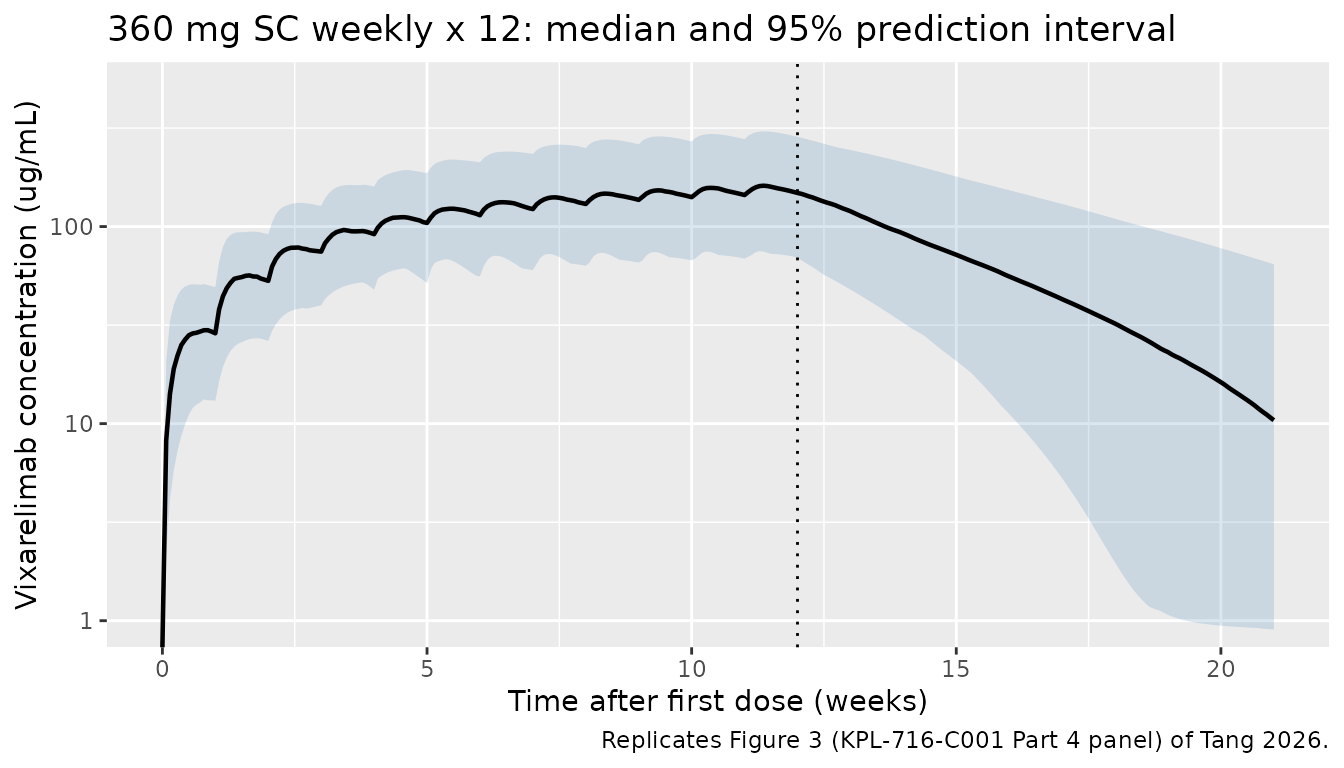
med_wk11 <- qw_sum$Q50[which.min(abs(qw_sum$time - WEEK * 11))]
# This IS a cohort-derived statistic, so the bound is deliberately loose. The
# median of 200 draws carries roughly 2% sampling error that varies with the
# solver thread count, and the published observed median in Figure 3 is read off
# a log axis as "roughly 150-200 ug/mL". Observed here: 141 ug/mL. The 100-250
# window still goes red for a mis-transcribed CL, dose or bioavailability, each
# of which moves this by tens of percent.
stopifnot(med_wk11 > 100, med_wk11 < 250)
c(simulated_median_week11_ug_per_mL = med_wk11)
#> simulated_median_week11_ug_per_mL
#>                          135.6996
Figure 4: body-weight effect on steady-state exposure
This is the paper’s sharpest quantitative answer key. Figure 4
reports the fold change in steady-state Cmax and
AUC0-tau after repeated 360 mg SC weekly dosing, for the
5th, 25th, 75th and 95th body-weight percentiles relative to a reference
participant weighing 82.1 kg, each with a 90% confidence interval from
500 simulations.
ss_interval <- function(wt, dose_mg, ii, n_doses = 60) {
  ev <- rxode2::et(amt = dose_mg, ii = ii, until = ii * (n_doses - 1), cmt = "depot") |>
    rxode2::et(seq(ii * (n_doses - 1), ii * n_doses, length.out = 400), cmt = "central")
  d <- as.data.frame(ev)
  d$WT <- wt
  rxode2::rxSolve(ui_typ, d, returnType = "data.frame", atol = 1e-10, rtol = 1e-8) |>
    dplyr::filter(!is.na(Cc))
}
trapz <- function(t, y) sum(diff(t) * (utils::head(y, -1) + utils::tail(y, -1)) / 2)

fig4_wt <- c(57.42, 69.1, 82.1, 94.5, 115.64)
fig4 <- do.call(rbind, lapply(fig4_wt, function(w) {
  s <- ss_interval(w, 360, WEEK)
  data.frame(WT = w, cmax = max(s$Cc), auc = trapz(s$time, s$Cc))
}))
#> ℹ omega/sigma items treated as zero: 'etalvc', 'etalcl', 'etalq', 'etalrbase', 'etalka', 'etalogitfdepot', 'etalvp'
#> ℹ omega/sigma items treated as zero: 'etalvc', 'etalcl', 'etalq', 'etalrbase', 'etalka', 'etalogitfdepot', 'etalvp'
#> ℹ omega/sigma items treated as zero: 'etalvc', 'etalcl', 'etalq', 'etalrbase', 'etalka', 'etalogitfdepot', 'etalvp'
#> ℹ omega/sigma items treated as zero: 'etalvc', 'etalcl', 'etalq', 'etalrbase', 'etalka', 'etalogitfdepot', 'etalvp'
#> ℹ omega/sigma items treated as zero: 'etalvc', 'etalcl', 'etalq', 'etalrbase', 'etalka', 'etalogitfdepot', 'etalvp'
ref4 <- fig4[fig4$WT == 82.1, ]
fig4$cmax_ratio <- fig4$cmax / ref4$cmax
fig4$auc_ratio  <- fig4$auc  / ref4$auc

published4 <- tibble::tribble(
  ~WT,     ~pub_cmax, ~cmax_lo, ~cmax_hi, ~pub_auc, ~auc_lo, ~auc_hi,
   57.42,   1.37,      1.31,     1.43,     1.38,     1.31,    1.45,
   69.10,   1.16,      1.14,     1.19,     1.17,     1.14,    1.20,
   94.50,   0.88,      0.86,     0.90,     0.88,     0.86,    0.90,
  115.64,   0.74,      0.70,     0.77,     0.73,     0.69,    0.76
)

fig4_cmp <- dplyr::inner_join(fig4, published4, by = "WT") |>
  dplyr::mutate(
    percentile = c("5th", "25th", "75th", "95th"),
    cmax_in_ci = cmax_ratio >= cmax_lo & cmax_ratio <= cmax_hi,
    auc_in_ci  = auc_ratio  >= auc_lo  & auc_ratio  <= auc_hi
  )

knitr::kable(
  fig4_cmp |>
    dplyr::transmute(
      percentile, WT,
      cmax_ratio,
      published_cmax = sprintf("%.2f [%.2f-%.2f]", pub_cmax, cmax_lo, cmax_hi),
      auc_ratio,
      published_auc = sprintf("%.2f [%.2f-%.2f]", pub_auc, auc_lo, auc_hi),
      cmax_in_ci, auc_in_ci
    ) |>
    dplyr::rename("Weight percentile" = percentile, "Weight (kg)" = WT,
                  "Simulated Cmax ratio" = cmax_ratio,
                  "Published Cmax [90% CI]" = published_cmax,
                  "Simulated AUC ratio" = auc_ratio,
                  "Published AUC [90% CI]" = published_auc,
                  "Cmax in CI" = cmax_in_ci, "AUC in CI" = auc_in_ci),
  digits = 3,
  caption = "Replicates Figure 4 of Tang 2026 (360 mg SC QW steady state, reference 82.1 kg)."
)| Weight percentile | Weight (kg) | Simulated Cmax ratio | Published Cmax [90% CI] | Simulated AUC ratio | Published AUC [90% CI] | Cmax in CI | AUC in CI |
|---|---|---|---|---|---|---|---|
| 5th | 57.42 | 1.420 | 1.37 [1.31-1.43] | 1.424 | 1.38 [1.31-1.45] | TRUE | TRUE |
| 25th | 69.10 | 1.185 | 1.16 [1.14-1.19] | 1.187 | 1.17 [1.14-1.20] | TRUE | TRUE |
| 75th | 94.50 | 0.870 | 0.88 [0.86-0.90] | 0.869 | 0.88 [0.86-0.90] | TRUE | TRUE |
| 95th | 115.64 | 0.711 | 0.74 [0.70-0.77] | 0.709 | 0.73 [0.69-0.76] | TRUE | TRUE |
stopifnot(
  # Every typical-value ratio falls inside the published 90% CI.
  all(fig4_cmp$cmax_in_ci),
  all(fig4_cmp$auc_in_ci),
  # Section 3.3: the 25th-75th percentile band lies inside 0.8-1.25.
  all(dplyr::filter(fig4_cmp, percentile %in% c("25th", "75th")) |>
        dplyr::summarise(ok = all(dplyr::c_across(c(cmax_ratio, auc_ratio)) > 0.8 &
                                  dplyr::c_across(c(cmax_ratio, auc_ratio)) < 1.25)) |>
        dplyr::pull(ok))
)
All eight simulated ratios fall inside the published 90% confidence intervals, and the 25th-75th percentile band lies within the 0.8-1.25 bioequivalence limits quoted in Section 3.3 – reproducing the paper’s conclusion that weight- based dose adjustment is not warranted.
Figure S6: free receptor occupancy
The Discussion states that “at 360 mg SC or 540 mg SC every 4 weeks, the levels of free receptors are predicted to be below 10% of the baseline level throughout the dosing interval, while 120 mg SC every 4 weeks is not expected to maintain sufficient target engagement.” Figure S6 plots this over the 16-week double-blind period of KPL-716-C201 Phase 2b.
Under the QSS approximation the free receptor concentration is
Rfree = Rtot * Kss / (Kss + Cfree).
q4w_doses <- c(120, 360, 540)
r0 <- exp(ui$theta[["lrbase"]])

s6 <- dplyr::bind_rows(lapply(q4w_doses, function(dose) {
  ev <- rxode2::et(amt = dose, ii = WEEK * 4, until = WEEK * 12, cmt = "depot") |>
    rxode2::et(seq(0, WEEK * 16, length.out = 2000), cmt = "central")
  d <- as.data.frame(ev)
  d$WT <- 82.1
  rxode2::rxSolve(ui_typ, d, returnType = "data.frame", atol = 1e-10, rtol = 1e-8) |>
    dplyr::filter(!is.na(Cc)) |>
    dplyr::transmute(time, dose = paste0(dose, " mg SC Q4W"),
                     free_receptor_pct = 100 * total_target * kss / (kss + cfree) / r0)
}))
#> ℹ omega/sigma items treated as zero: 'etalvc', 'etalcl', 'etalq', 'etalrbase', 'etalka', 'etalogitfdepot', 'etalvp'
#> ℹ omega/sigma items treated as zero: 'etalvc', 'etalcl', 'etalq', 'etalrbase', 'etalka', 'etalogitfdepot', 'etalvp'
#> ℹ omega/sigma items treated as zero: 'etalvc', 'etalcl', 'etalq', 'etalrbase', 'etalka', 'etalogitfdepot', 'etalvp'

ggplot(s6, aes(time / WEEK, free_receptor_pct, colour = dose)) +
  geom_line(linewidth = 0.8) +
  geom_hline(yintercept = 10, linetype = "dashed") +
  labs(x = "Time (weeks)", y = "Free receptor (% baseline)", colour = NULL,
       title = "Predicted typical free OSMR-beta over the 16-week double-blind period",
       caption = "Replicates Figure S6 of Tang 2026. Dashed line = 10% of baseline.")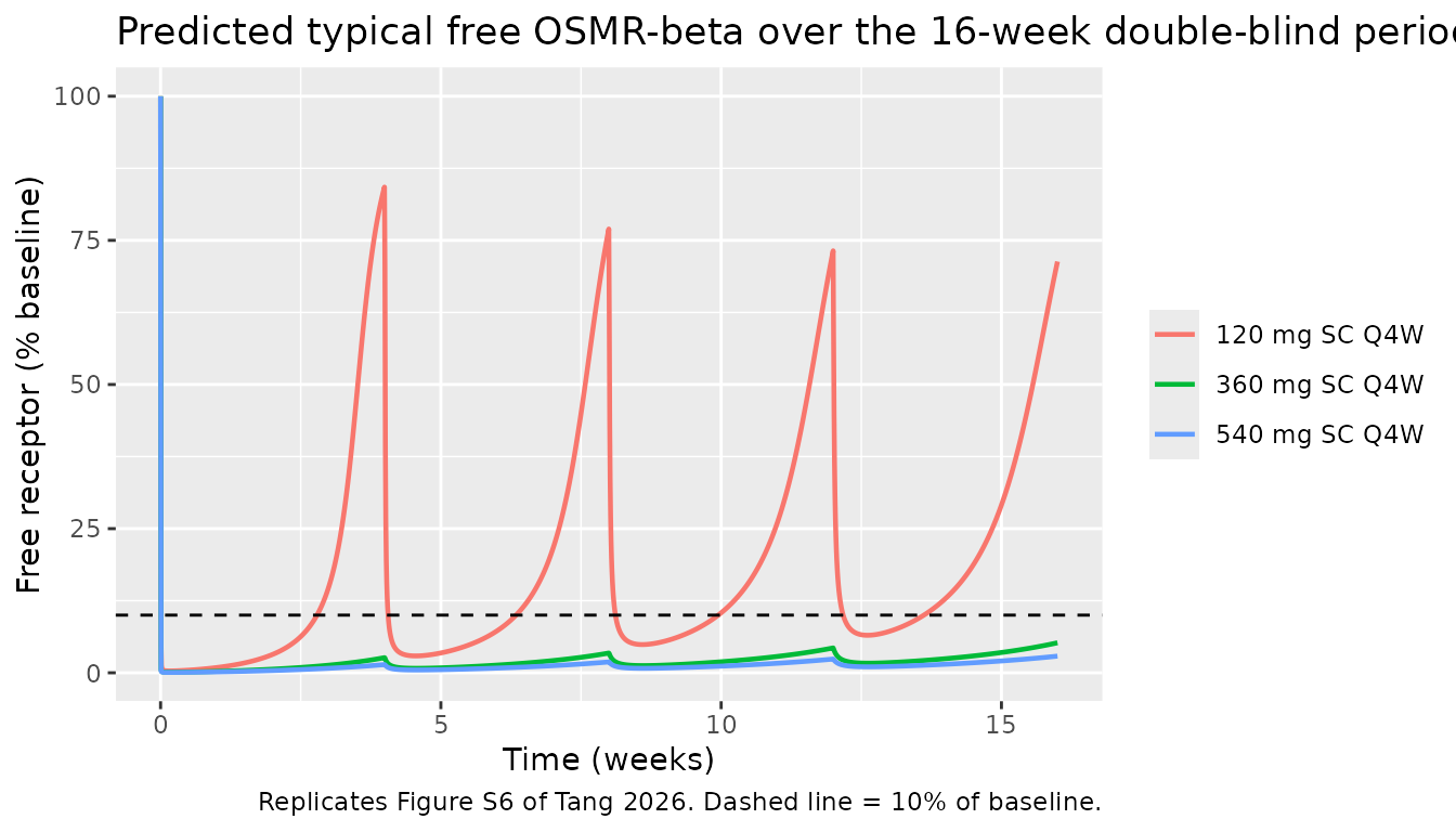
# Exclude the pre-dose transient (the profile starts at 100% by construction).
s6_peak <- s6 |>
  dplyr::filter(time >= WEEK) |>
  dplyr::group_by(dose) |>
  dplyr::summarise(peak_pct = max(free_receptor_pct), .groups = "drop")

knitr::kable(
  s6_peak |> dplyr::rename("Regimen" = dose, "Peak free receptor (% baseline)" = peak_pct),
  digits = 1, caption = "Peak free receptor after the first week of dosing."
)| Regimen | Peak free receptor (% baseline) |
|---|---|
| 120 mg SC Q4W | 84.2 |
| 360 mg SC Q4W | 5.2 |
| 540 mg SC Q4W | 2.9 |
stopifnot(
  # 360 and 540 mg Q4W hold free receptor below 10% of baseline throughout.
  s6_peak$peak_pct[s6_peak$dose == "360 mg SC Q4W"] < 10,
  s6_peak$peak_pct[s6_peak$dose == "540 mg SC Q4W"] < 10,
  # 120 mg Q4W does not -- it recovers to most of baseline before each dose.
  s6_peak$peak_pct[s6_peak$dose == "120 mg SC Q4W"] > 50
)
Structural identity: drug mass balance
For an exact check that Equations 2-6 are transcribed correctly, the dose must be fully accounted for by the two elimination routes plus whatever drug is left in the body. Both sides use the same drawn parameters, so this is pure numerical error and a tight bound is appropriate.
ev_mb <- rxode2::et(amt = 360, cmt = "depot") |>
  rxode2::et(seq(0, WEEK * 60, length.out = 40000), cmt = "central")
d_mb <- as.data.frame(ev_mb)
d_mb$WT <- 82.1
mb <- rxode2::rxSolve(ui_typ, d_mb, returnType = "data.frame", atol = 1e-12, rtol = 1e-10) |>
  dplyr::filter(!is.na(Cc))
#> ℹ omega/sigma items treated as zero: 'etalvc', 'etalcl', 'etalq', 'etalrbase', 'etalka', 'etalogitfdepot', 'etalvp'

complex_conc <- mb$ctot - mb$cfree
eliminated_linear <- mb$cl[1] * trapz(mb$time, mb$cfree)
eliminated_target <- mb$kint[1] * mb$vc[1] * trapz(mb$time, complex_conc)
remaining <- utils::tail(mb$depot, 1) + utils::tail(mb$central, 1) +
  utils::tail(mb$peripheral1, 1)
dose_nmol <- mb$fdepot[1] * 360 * 1e6 / 150000

closure <- abs(dose_nmol - (eliminated_linear + eliminated_target + remaining)) / dose_nmol
target_share <- eliminated_target / (eliminated_linear + eliminated_target)

stopifnot(closure < 1e-6)
c(bioavailable_dose_nmol = dose_nmol,
  linear_route_nmol = eliminated_linear,
  target_mediated_route_nmol = eliminated_target,
  relative_closure_error = closure,
  target_mediated_share_of_elimination = target_share)
#>               bioavailable_dose_nmol                    linear_route_nmol
#>                         1.358400e+03                         8.131053e+02
#>           target_mediated_route_nmol               relative_closure_error
#>                         4.175133e+02                         4.944268e-09
#> target_mediated_share_of_elimination
#>                         3.392711e-01
The mass balance closes to better than one part in a million, and
roughly a third of a single 360 mg SC dose is cleared through the
target-mediated route – which is why the apparent clearance in the NCA
table above sits above the linear CL even at 20 mg/kg.
Molecular-weight sensitivity
The packaged model converts mg to nmol with a nominal IgG molecular weight of 150 000 g/mol, because vixarelimab’s molecular weight is not reported in the paper or its Supporting Information (see Assumptions and deviations). This matters only for the nonlinear arm: once the target is saturated, the model reduces to a linear two-compartment system whose mass-unit predictions are exactly molecular-weight-invariant, because the factor cancels between the dose conversion and the observation conversion. At the clinically relevant 360 mg weekly regimen this leaves very little residual sensitivity.
# `rxode2::model()` piping rewrites the single `mw <- ...` line in the packaged
# model, so the sensitivity analysis needs no file surgery.
cavg_at_mw <- function(mw_value) {
  m <- rxode2::zeroRe(eval(bquote(rxode2::model(ui, mw <- .(mw_value)))))
  ev <- rxode2::et(amt = 360, ii = WEEK, until = WEEK * 59, cmt = "depot") |>
    rxode2::et(seq(WEEK * 59, WEEK * 60, length.out = 400), cmt = "central")
  d <- as.data.frame(ev)
  d$WT <- 82.1
  s <- rxode2::rxSolve(m, d, returnType = "data.frame", atol = 1e-10, rtol = 1e-8) |>
    dplyr::filter(!is.na(Cc))
  trapz(s$time, s$Cc) / WEEK
}

mw_grid <- c(130000, 140000, 150000, 160000, 170000)
cavg <- vapply(mw_grid, cavg_at_mw, numeric(1))
#> ℹ omega/sigma items treated as zero: 'etalvc', 'etalcl', 'etalq', 'etalrbase', 'etalka', 'etalogitfdepot', 'etalvp'
#> ℹ omega/sigma items treated as zero: 'etalvc', 'etalcl', 'etalq', 'etalrbase', 'etalka', 'etalogitfdepot', 'etalvp'
#> ℹ omega/sigma items treated as zero: 'etalvc', 'etalcl', 'etalq', 'etalrbase', 'etalka', 'etalogitfdepot', 'etalvp'
#> ℹ omega/sigma items treated as zero: 'etalvc', 'etalcl', 'etalq', 'etalrbase', 'etalka', 'etalogitfdepot', 'etalvp'
#> ℹ omega/sigma items treated as zero: 'etalvc', 'etalcl', 'etalq', 'etalrbase', 'etalka', 'etalogitfdepot', 'etalvp'
mw_tab <- data.frame(mw_g_per_mol = mw_grid, cavg_ug_per_mL = cavg,
                     pct_vs_150k = 100 * (cavg / cavg[mw_grid == 150000] - 1))

knitr::kable(
  mw_tab |>
    dplyr::rename("Molecular weight (g/mol)" = mw_g_per_mol,
                  "Steady-state Cavg (ug/mL)" = cavg_ug_per_mL,
                  "Difference vs 150 kDa (%)" = pct_vs_150k),
  digits = c(0, 2, 2),
  caption = "Steady-state Cavg at 360 mg SC weekly across a +/-13% molecular-weight range."
)| Molecular weight (g/mol) | Steady-state Cavg (ug/mL) | Difference vs 150 kDa (%) |
|---|---|---|
| 130000 | 175.28 | 0.94 |
| 140000 | 174.47 | 0.47 |
| 150000 | 173.65 | 0.00 |
| 160000 | 172.84 | -0.47 |
| 170000 | 172.03 | -0.94 |
A +/-13% change in the assumed molecular weight moves
steady-state Cavg by less than 2%, so the assumption does
not materially affect the exposures the model is used to predict. For
comparison, the fully linear closed form
F * Dose / (CL * tau) gives 186.9 ug/mL, about 7% above the
simulated 173.7 ug/mL – the difference being the drug still lost through
the target-mediated route at steady state.
Assumptions and deviations
-
Molecular weight (non-paper value). The authors’
model is entirely molar:
R0andKssare estimated in nM and Equation 6 subtracts them from the drug concentration. Their deposited$INPUTcarries both mass columns (AMTMG,DVUGML) and molar columns (AMT,DVNM), so the mg-to-nmol conversion was done in their SAS derivation, but the conversion factor itself is not reported in the paper or the Supporting Information. The packaged model uses the nominal molecular weight of a human IgG monoclonal antibody, 150 000 g/mol, following the same convention asinst/modeldb/specificDrugs/Papachristos_2020_bevacizumab_qss.R. The molecular-weight sensitivity section above bounds the consequence at under 2% for the 360 mg weekly regimen. A user with the true molecular weight can edit the singlemw <- 150000line in the model file. -
Body-weight centring constant. The 81.7 kg
reference weight appears only in the deposited control stream
(
(WT/81.7)**THETA(11)), not in the paper text. It is consistent with the cohort median of 82 kg (Table 2). Figure 4 separately describes its reference participant as weighing 82.1 kg; that value is used for the Figure 4 replication above, and 81.7 kg is used for the covariate model itself, matching the two sources. -
Table S3 erratum. Table S3 describes run 7 (the
final model) as “Removing IIV on Q”. This contradicts three agreeing
sources: Section 3.2 (“the estimated IIV on Vp approached 0 and was
poorly estimated. Fixing the IIV on Vp to 0 had no change in the OFV and
yielded the final model”), Table 3 (which reports a between-subject
variability for Q of 91.6% but none for Vp), and the deposited
$OMEGAblock (0.609013 ; ETA_Qalongside0 FIX ; ETA_VP). The packaged model follows the three agreeing sources: IIV is estimated on Q and fixed to zero on Vp. -
Control-stream
$THETArecords are initial, not final, estimates. Nine of the eleven$THETAvalues in the deposited run-7 stream match Table 3 to the printed precision, butPOPVC(2.9 vs 3.04) andPOPKINT(0.000146168 vs 0.000141) do not. All packaged values are taken from Table 3, the published final-model table. -
Dead code in the control stream. The
$PKblock containsIF(ROUTE.EQ.1) KA = 0, which is immediately overwritten byKA = TVKA * EXP(ETA(9))four lines later, so it never takes effect. It is not reproduced. Intravenous dosing is handled by dosing directly intocentral, which leaves the depot empty regardless ofKa. -
IIV variances are back-transformed from Table 3’s
CV%. Table 3 reports variability only as
CV% = sqrt(exp(omega^2) - 1) * 100%, so the packaged variances areomega^2 = log(1 + (CV/100)^2). These agree with the deposited$OMEGAdiagonal to within 0.3%. Note that the CV% transform is applied by the authors to the F1 variability too, even thoughETA(10)is additive on the logit scale, where a log-normal CV is not a meaningful summary; the packaged model carries the variance, not the CV. -
Screened but unretained covariates. Age, sex, race
(Asian versus others), ADA status and healthy-volunteer-versus-patient
status were pre-specified and tested (Table S2) but not retained in the
final model, and no point estimates are published for them. They are
recorded in the model file’s
covariatesDataExcludedlist for provenance and are not referenced inmodel(). - Virtual cohort. Only body weight enters the final model, so cohorts are built by drawing weights from a log-normal distribution matched to the Table 2 median of 82 kg and truncated to the observed 48-158 kg range. No attempt is made to reproduce the joint age/sex/race distribution, since none of those covariates affects the model.
-
No published NCA table. The source reports no
non-compartmental Cmax / Tmax / AUC / half-life values, so there is no
nlmixr2lib::ncaComparisonTable()comparison here. PKNCA is instead used to test the paper’s quantitative claims about the dose-dependence of exposure (Section 3.1 and Figure S1). - Apparent half-life definition. PKNCA’s automatic lambda-z selection returns unstable values for this model because the log-concentration profile is genuinely curved under target-mediated elimination. The apparent terminal half-life is therefore defined explicitly as the slope of a log-linear fit over the whole quantifiable post-distribution profile.