Methotrexate (Blackman 2026)

Model and source

• Citation: Blackman MH, Yelvington B, Beck C, Cortez M, Choi L. (2026). Development and validation of high-dose methotrexate population pharmacokinetic models to inform clinical decisions on dosing. Eur J Clin Pharmacol 82:156. doi:10.1007/s00228-026-04080-0.
• Description: Three-compartment population PK model for high-dose intravenous methotrexate in adult patients with leukemia, lymphoma, or sarcoma treated at Vanderbilt University Medical Center (Blackman 2026), with body surface area on all six disposition parameters (an estimated exponent on clearance and an exponent fixed at 1 on the central and peripheral volumes and both inter-compartmental clearances), serum creatinine and female sex as additional covariates on clearance, inter-individual variability on all six PK parameters, four-occasion inter-occasion variability on clearance, and proportional residual error. Parameter values are taken from the publication’s Table 2 (Final Model column).
• Article: https://doi.org/10.1007/s00228-026-04080-0

Blackman and colleagues developed a three-compartment population PK model for high-dose methotrexate (HD-MTX) in adults, then benchmarked it against ten previously published models on a held-out test set. Only the authors’ own final model is packaged here. The ten comparator models are other groups’ publications that Blackman 2026 re-implemented for evaluation; Table 3 of the paper records their structure but not their parameter values, so they are not extractable from this source. Two of them are already in nlmixr2lib in their own right – modellib("Taylor_2020_methotrexate") and modellib("Olivo_2024_methotrexate").

The paper reports three nested models (base, BSA-adjusted, and final). Following the library’s replicate-the-author’s-structure policy, only the Final Model column of Table 2 is packaged; the base and BSA-adjusted columns are development stages rather than reported results.

Population

The model was fit to the training subset of an electronic-health-record cohort of 208 adults who received an HD-MTX-containing regimen at Vanderbilt University Medical Center between November 2017 and December 2022. The 208 patients were split randomly 70:30, giving N = 145 training patients (the fit this file packages) and N = 63 test patients used only for validation.

Training-set characteristics (Table 1): median age 56 years (range 18-84), 60.0% female, median weight 82.4 kg (42.4-141.0), median body surface area 1.97 m^2 (1.32-2.66), and median serum creatinine 68.5 umol/L (44.2-132). Indications were lymphoma (51.0%), leukemia (40.7%) and sarcoma (6.9%). Excluding loading doses the median dose was 3.5 g/m^2 (range 0.2-12.1) infused over a median of 4.7 h (range 2.0-27.9); infusions were given as short-term single doses (59%), long-term single doses (19%), or a loading dose plus maintenance (22%), at intervals of typically 2-4 weeks. Patients contributed a median of 9 drug levels and 4 dosing events across a median of 3 cycles. Patients who received glucarpidase were excluded because it alters methotrexate clearance; all patients received leucovorin rescue beginning 24 h after dosing, which the model does not represent.

The same information is available programmatically:

pop <- rxode2::rxode(readModelDb("Blackman_2026_methotrexate"))$population
#> ℹ parameter labels from comments will be replaced by 'label()'
#> Warning: some etas defaulted to non-mu referenced, possible parsing error: etaiov_cl_1, etaiov_cl_2, etaiov_cl_3, etaiov_cl_4
#> as a work-around try putting the mu-referenced expression on a simple line
str(pop, max.level = 1)
#> List of 15
#>  $ species       : chr "human"
#>  $ n_subjects    : int 145
#>  $ n_studies     : int 1
#>  $ age_range     : chr "18-84 years (median 56)"
#>  $ age_median    : chr "56 years"
#>  $ weight_range  : chr "42.4-141.0 kg (median 82.4)"
#>  $ weight_median : chr "82.4 kg"
#>  $ bsa_range     : chr "1.32-2.66 m^2 (median 1.97)"
#>  $ bsa_median    : chr "1.97 m^2"
#>  $ sex_female_pct: num 60
#>  $ renal_function: chr "Serum creatinine 44.2-132 umol/L (median 68.5). Patients who received glucarpidase were excluded because it alt"| __truncated__
#>  $ disease_state : chr "Adults receiving a high-dose methotrexate-containing regimen for lymphoma (51.0%), leukemia (40.7%), or sarcoma"| __truncated__
#>  $ dose_range    : chr "Intravenous methotrexate 200 mg/m^2 or higher; excluding loading doses the training-set dose was a median of 3."| __truncated__
#>  $ regions       : chr "United States (single center: Vanderbilt University Medical Center), November 2017 through December 2022."
#>  $ notes         : chr "Electronic-health-record cohort of 208 adults split randomly 70:30 into training (N = 145) and test (N = 63) da"| __truncated__

Source trace

Every ini() entry in inst/modeldb/specificDrugs/Blackman_2026_methotrexate.R carries an in-file comment naming its origin. They are collected here for review. All parameter values come from the Final Model column of Table 2 (OFV = -2512.1, AIC = -2478.1, BIC = -2407.3).

Equation / parameter	Value	Source location
lcl (CL)	9.41 L/h	Table 2, Final Model, theta1 (SE 0.37)
lvc (V1)	30.67 L	Table 2, Final Model, theta2 (SE 1.42)
lq (Q2)	0.87 L/h	Table 2, Final Model, theta3 (SE 0.07)
lvp (V2)	5.62 L	Table 2, Final Model, theta4 (SE 0.29)
lq2 (Q3)	0.14 L/h	Table 2, Final Model, theta5 (SE 0.01)
lvp2 (V3)	10.60 L	Table 2, Final Model, theta6 (SE 2.43)
e_bsa_cl	0.61	Table 2, Final Model, theta7 (SE 0.14)
e_creat_cl	-0.56	Table 2, Final Model, theta8 (SE 0.08)
e_sexf_cl	0.01	Table 2, Final Model, theta9 (SE 0.05)
e_bsa_vc, e_bsa_q, e_bsa_vp, e_bsa_q2, e_bsa_vp2	1 (fixed)	Methods “Population PK analysis”; superscript 1 on the V1/Q2/V2/Q3/V3 rows of Table 2
etalcl	0.24^2	Table 2, Final Model, omegaCL (SE 0.02)
etalvc	0.29^2	Table 2, Final Model, omegaV1 (SE 0.03)
etalq	0.38^2	Table 2, Final Model, omegaQ2 (SE 0.12)
etalvp	0.30^2	Table 2, Final Model, omegaV2 (SE 0.05)
etalq2	0.47^2	Table 2, Final Model, omegaQ3 (SE 0.05)
etalvp2	0.34^2	Table 2, Final Model, omegaV3 (SE 0.28)
etaiov_cl_1 .. _4	0.14^2	Table 2, Final Model, deltaCL (SE 0.01)
propSd	0.25	Table 2, Final Model, sigma_proportional (SE 0.01)
CL covariate equation	n/a	Table 2 Final Model header row and the Results display equation for CL_ij
V1/Q2/V2/Q3/V3 BSA equations	n/a	Table 2 Final Model header rows and the Results display equations
Three-compartment IV disposition	n/a	Results “Population PK model” paragraph 1 (CL, V1, Q2, V2, Q3, V3 parameterisation)
Proportional residual error	n/a	Results “Population PK model”: “base model was a three-compartment model with proportional error”
Reference BSA 1.97 m^2, SCR 68.08 umol/L	n/a	Table 2 Final Model equations; BSA matches the Table 1 median

Random-effect scale

Table 2 heads the variability rows omega<param> (%CV) without stating whether the tabulated number is a standard deviation or a variance. Three independent lines of evidence establish that they are lognormal SDs on the log scale, so the model file squares them for nlmixr2’s variance parameterisation.

omega_sd <- c(CL = 0.24, V1 = 0.29, Q2 = 0.38, V2 = 0.30, Q3 = 0.47, V3 = 0.34)
# The Results text quotes these same six numbers as percent CV:
paper_cv <- c(CL = 24, V1 = 29, Q2 = 38, V2 = 30, Q3 = 47, V3 = 34)

as_sd  <- sqrt(exp(omega_sd^2) - 1) * 100   # reading the entry as an SD
as_var <- sqrt(exp(omega_sd) - 1) * 100     # reading the entry as a variance

data.frame(
  parameter          = names(omega_sd),
  `Table 2 entry`    = omega_sd,
  `Paper %CV`        = paper_cv,
  `CV if SD`         = round(as_sd, 1),
  `CV if variance`   = round(as_var, 1),
  check.names = FALSE
) |>
  knitr::kable(caption = "Only the SD reading reproduces the percent CVs quoted in the Results text.")

Only the SD reading reproduces the percent CVs quoted in the Results text.

	parameter	Table 2 entry	Paper %CV	CV if SD	CV if variance
CL	CL	0.24	24	24.3	52.1
V1	V1	0.29	29	29.6	58.0
Q2	Q2	0.38	38	39.4	68.0
V2	V2	0.30	30	30.7	59.1
Q3	Q3	0.47	47	49.7	77.5
V3	V3	0.34	34	35.0	63.6

# The SD reading is within a couple of points of the quoted CV for every
# parameter; the variance reading is off by a factor approaching two.
stopifnot(
  max(abs(as_sd  - paper_cv)) <  4,
  min(abs(as_var - paper_cv)) > 15
)

A second, independent check comes from the reported standard errors. A variance estimated on N = 145 subjects cannot have a relative standard error much below sqrt(2 / N); the reported omegaCL = 0.24 (SE 0.02) is an 8.3% RSE, comfortably under that floor and therefore an SD.

rse_floor <- sqrt(2 / 145) * 100
c(`omegaCL RSE (%)` = 0.02 / 0.24 * 100, `variance RSE floor (%)` = rse_floor) |>
  round(1)
#>        omegaCL RSE (%) variance RSE floor (%) 
#>                    8.3                   11.7
stopifnot(0.02 / 0.24 * 100 < rse_floor)

Structural verification

Before simulating a cohort, two deterministic checks confirm the transcription. Both compare quantities that share the same parameter draw, so the only difference is numerical error and a tight bound is the correct assertion.

Three-compartment solve against its closed form

ui  <- rxode2::rxode(readModelDb("Blackman_2026_methotrexate"))
#> ℹ parameter labels from comments will be replaced by 'label()'
#> Warning: some etas defaulted to non-mu referenced, possible parsing error: etaiov_cl_1, etaiov_cl_2, etaiov_cl_3, etaiov_cl_4
#> as a work-around try putting the mu-referenced expression on a simple line
uiz <- rxode2::zeroRe(ui)
#> Warning: some etas defaulted to non-mu referenced, possible parsing error: etaiov_cl_1, etaiov_cl_2, etaiov_cl_3, etaiov_cl_4
#> as a work-around try putting the mu-referenced expression on a simple line

cl <- 9.41; vc <- 30.67; q <- 0.87; vp <- 5.62; q2 <- 0.14; vp2 <- 10.60
k10 <- cl / vc; k12 <- q / vc; k21 <- q / vp; k13 <- q2 / vc; k31 <- q2 / vp2

amat <- matrix(
  c(-(k10 + k12 + k13), k21,  k31,
    k12,               -k21,  0,
    k13,                0,   -k31),
  nrow = 3, byrow = TRUE
)
eg  <- eigen(amat)
amt <- 1000
cf  <- solve(eg$vectors, c(amt, 0, 0))

tgrid <- seq(0.1, 96, by = 0.1)
analytic <- vapply(
  tgrid,
  function(tt) Re(sum(eg$vectors[1, ] * cf * exp(eg$values * tt))),
  numeric(1)
) / vc

ev_bolus <- rxode2::et(amt = amt, cmt = "central") |>
  rxode2::et(tgrid, cmt = "central")
d_bolus <- as.data.frame(ev_bolus)
d_bolus$BSA <- 1.97; d_bolus$CREAT <- 68.08; d_bolus$SEXF <- 0; d_bolus$OCC <- 1L

numeric_sol <- rxode2::rxSolve(uiz, d_bolus, returnType = "data.frame")
#> Warning: some etas defaulted to non-mu referenced, possible parsing error: etaiov_cl_1, etaiov_cl_2, etaiov_cl_3, etaiov_cl_4
#> as a work-around try putting the mu-referenced expression on a simple line
#> ℹ omega/sigma items treated as zero: 'etalcl', 'etalvc', 'etalq', 'etalvp', 'etalq2', 'etalvp2', 'etaiov_cl_1', 'etaiov_cl_2', 'etaiov_cl_3', 'etaiov_cl_4'
numeric_sol <- numeric_sol$Cc[match(round(tgrid, 4), round(numeric_sol$time, 4))]

max_rel <- max(abs(numeric_sol - analytic) / analytic)
cat(sprintf("max |relative difference| = %.3e\n", max_rel))
#> max |relative difference| = 2.608e-14

# Both sides use the same parameters, so this is pure integration error.
stopifnot(max_rel < 1e-6)

The eigenvalues give the model’s three disposition half-lives, which are a property of the packaged parameters rather than a published quantity:

hl <- sort(log(2) / -Re(eg$values))
setNames(round(hl, 2), c("t1/2 alpha (h)", "t1/2 beta (h)", "t1/2 gamma (h)"))
#> t1/2 alpha (h)  t1/2 beta (h) t1/2 gamma (h) 
#>           1.92           5.19          53.30

The deep third compartment (Q3 = 0.14 L/h into V3 = 10.60 L) governs a terminal half-life near 53 h, which is what makes methotrexate elimination monitoring run out to 72 h and beyond.

Covariate equation against the published closed form

# Table 2 Final Model:
#   CL = theta1 * (BSA/1.97)^theta7 * (SCR/68.08)^theta8 * exp(theta9 * I(female))
published_cl <- function(bsa, scr, sexf) {
  9.41 * (bsa / 1.97)^0.61 * (scr / 68.08)^(-0.56) * exp(0.01 * sexf)
}

grid_cov <- expand.grid(
  BSA   = c(1.4, 1.97, 2.6),
  CREAT = c(45, 68.08, 130),
  SEXF  = c(0, 1)
)
grid_cov$OCC <- 1L
grid_cov$id  <- seq_len(nrow(grid_cov))

ev_cov <- grid_cov |>
  tidyr::crossing(time = c(0, 1)) |>
  dplyr::mutate(evid = 0L, amt = NA_real_, cmt = "central") |>
  dplyr::arrange(id, time)

sim_cov <- rxode2::rxSolve(uiz, ev_cov, returnType = "data.frame") |>
  dplyr::distinct(id, .keep_all = TRUE)
#> ℹ omega/sigma items treated as zero: 'etalcl', 'etalvc', 'etalq', 'etalvp', 'etalq2', 'etalvp2', 'etaiov_cl_1', 'etaiov_cl_2', 'etaiov_cl_3', 'etaiov_cl_4'
#> Warning: multi-subject simulation without without 'omega'

# rxSolve returns the input covariate columns directly, so no join is needed
# here -- joining `grid_cov` back on would produce BSA.x / BSA.y and lose `BSA`.
stopifnot(all(c("BSA", "CREAT", "SEXF", "cl") %in% names(sim_cov)))

chk_cl <- sim_cov |>
  dplyr::mutate(expected = published_cl(BSA, CREAT, SEXF),
                rel = abs(cl - expected) / expected)

stopifnot(nrow(chk_cl) == nrow(grid_cov), max(chk_cl$rel) < 1e-8)
cat(sprintf("CL matches the published closed form at all %d covariate combinations (max rel. diff %.2e)\n",
            nrow(chk_cl), max(chk_cl$rel)))
#> CL matches the published closed form at all 18 covariate combinations (max rel. diff 2.02e-15)

The covariate effects, expressed as the change in clearance across the observed covariate range, are:

data.frame(
  Covariate = c("BSA 1.32 -> 2.66 m^2 (Table 1 range)",
                "SCR 44.2 -> 132 umol/L (Table 1 range)",
                "Male -> female"),
  `Fold change in CL` = round(c(
    (2.66 / 1.32)^0.61,
    (132 / 44.2)^(-0.56),
    exp(0.01)
  ), 3),
  check.names = FALSE
) |>
  knitr::kable(caption = "Clearance effect sizes over the cohort covariate ranges.")

Clearance effect sizes over the cohort covariate ranges.

Covariate	Fold change in CL
BSA 1.32 -> 2.66 m^2 (Table 1 range)	1.533
SCR 44.2 -> 132 umol/L (Table 1 range)	0.542
Male -> female	1.010

Serum creatinine is by far the strongest covariate: a patient at the top of the observed SCR range clears methotrexate at roughly half the rate of one at the bottom. Sex, by contrast, changes clearance by 1% – see the Errata section.

Virtual cohort

The original observations are not public (the paper’s data-availability statement cites IRB and consent restrictions), so the figures below use a virtual cohort whose covariate distributions approximate the Table 1 training-set demographics.

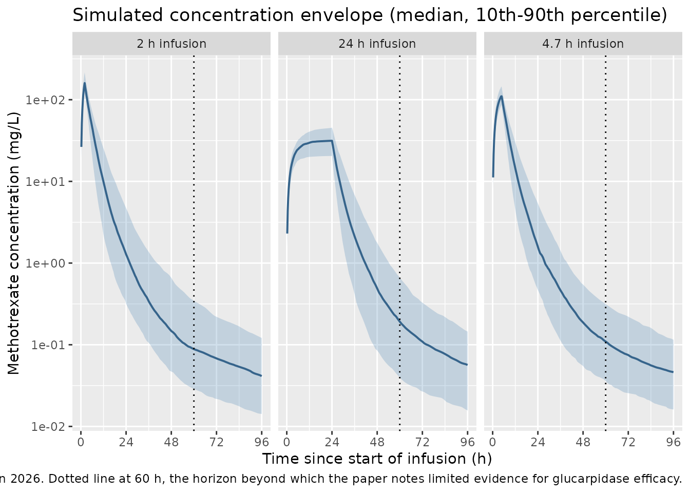
The 24 h concentration is strongly dependent on infusion duration, and the cohort pooled short-term (59%), long-term (19%) and loading-plus-maintenance (22%) regimens. Three arms are therefore simulated at the Table 1 median dose of 3.5 g/m^2, spanning the reported infusion-duration range of 2.0-27.9 h.

# Truncated normal sampler, resampling the out-of-range draws. Defined at top
# level rather than nested inside make_cohort().
rtrunc_norm <- function(n, mean, sd, lo, hi) {
  x <- stats::rnorm(n, mean, sd)
  bad <- x < lo | x > hi
  while (any(bad)) {
    x[bad] <- stats::rnorm(sum(bad), mean, sd)
    bad <- x < lo | x > hi
  }
  x
}

obs_times <- sort(unique(c(
  seq(0, 30, by = 0.25),
  seq(31, 96, by = 1),
  24, 48, 72
)))

make_cohort <- function(n, dur_h, arm, id_offset = 0L, dose_gm2 = 3.5) {
  subj <- tibble::tibble(
    id    = id_offset + seq_len(n),
    # Table 1 training set: BSA mean 1.97 (SD 0.28), range 1.32-2.66 m^2
    BSA   = rtrunc_norm(n, 1.97, 0.28, 1.32, 2.66),
    # Table 1 training set: SCR mean 72.5 (SD 16.4), range 44.2-132 umol/L
    CREAT = rtrunc_norm(n, 72.5, 16.4, 44.2, 132),
    # Table 1 training set: 60.0% female
    SEXF  = stats::rbinom(n, 1L, 0.60),
    OCC   = 1L,
    arm   = arm
  ) |>
    dplyr::mutate(dose_mg = dose_gm2 * BSA * 1000)

  dosing <- subj |>
    dplyr::mutate(time = 0, evid = 1L, amt = dose_mg,
                  dur = dur_h, cmt = "central")

  obs <- subj |>
    tidyr::crossing(time = obs_times) |>
    dplyr::mutate(evid = 0L, amt = NA_real_,
                  dur = NA_real_, cmt = "central")

  dplyr::bind_rows(dosing, obs) |>
    dplyr::arrange(id, time, dplyr::desc(evid)) |>
    dplyr::select(id, time, evid, amt, dur, cmt,
                  BSA, CREAT, SEXF, OCC, arm, dose_mg)
}

# set.seed() seeds R's RNG (the covariate draws below). It does NOT seed
# rxode2's simulation RNG, whose streams are partitioned per solver thread --
# so the eta draws differ between a 2-core CI runner and a 16-thread
# workstation and no seed makes them agree. Every assertion downstream is
# written to hold for any cohort this model can produce.
set.seed(20260901)

n_arm <- 200L  # <= 200 per arm

events <- dplyr::bind_rows(
  make_cohort(n_arm,  2.0, "2 h infusion",    id_offset =   0L),
  make_cohort(n_arm,  4.7, "4.7 h infusion",  id_offset = 200L),
  make_cohort(n_arm, 24.0, "24 h infusion",   id_offset = 400L)
)

# Disjoint IDs across arms: duplicate IDs silently merge into one subject
# receiving the summed dose.
stopifnot(!anyDuplicated(unique(events[, c("id", "time", "evid")])))
stopifnot(dplyr::n_distinct(events$id) == 3L * n_arm)

Simulation

mod <- readModelDb("Blackman_2026_methotrexate")

sim <- rxode2::rxSolve(mod, events = events, keep = c("arm", "dose_mg")) |>
  as.data.frame()
#> ℹ parameter labels from comments will be replaced by 'label()'
#> Warning: some etas defaulted to non-mu referenced, possible parsing error: etaiov_cl_1, etaiov_cl_2, etaiov_cl_3, etaiov_cl_4
#> as a work-around try putting the mu-referenced expression on a simple line
#> Warning: some etas defaulted to non-mu referenced, possible parsing error: etaiov_cl_1, etaiov_cl_2, etaiov_cl_3, etaiov_cl_4
#> as a work-around try putting the mu-referenced expression on a simple line

# rxSolve returns ONE ROW PER OBSERVATION RECORD and carries no `evid` column,
# so nothing downstream may filter on `evid`; the dose rows are already gone.
stopifnot(all(c("Cc", "cl", "arm", "BSA", "CREAT") %in% names(sim)))
stopifnot(!("evid" %in% names(sim)))
stopifnot(nrow(sim) == 3L * n_arm * length(obs_times))
stopifnot(all(sim$Cc >= 0, na.rm = TRUE))

Replicate published figures

Figure 1A (observed vs predicted) and Figure 1B (individual weighted residuals) of Blackman 2026 both require the observed test-set concentrations, which are not public, so they cannot be reproduced. Figure 1C is a visual predictive check; the plot below is its simulation-only counterpart.

# Analogous to Figure 1C of Blackman 2026: concentration-time envelope over the
# 0-96 h window the paper modelled, with the 60 h horizon it highlights as the
# clinically decisive period for glucarpidase.
vpc <- sim |>
  # Drop the time-zero row only because the log scale cannot show it. This is a
  # plotting filter; the PKNCA input below deliberately keeps time zero.
  dplyr::filter(time != 0) |>
  dplyr::group_by(arm, time) |>
  dplyr::summarise(
    Q10 = quantile(Cc, 0.10),
    Q50 = quantile(Cc, 0.50),
    Q90 = quantile(Cc, 0.90),
    .groups = "drop"
  )

ggplot(vpc, aes(time, Q50)) +
  geom_ribbon(aes(ymin = Q10, ymax = Q90), alpha = 0.25, fill = "steelblue") +
  geom_line(colour = "steelblue4", linewidth = 0.7) +
  geom_vline(xintercept = 60, linetype = "dotted") +
  facet_wrap(~arm) +
  scale_y_log10() +
  scale_x_continuous(breaks = c(0, 24, 48, 72, 96)) +
  labs(
    x = "Time since start of infusion (h)",
    y = "Methotrexate concentration (mg/L)",
    title = "Simulated concentration envelope (median, 10th-90th percentile)",
    caption = paste("Counterpart to Figure 1C of Blackman 2026. Dotted line at 60 h,",
                    "the horizon beyond which the paper notes limited evidence",
                    "for glucarpidase efficacy.")
  )

# The paper's covariate contribution: clearance against BSA and serum creatinine.
sim |>
  dplyr::distinct(id, .keep_all = TRUE) |>
  dplyr::select(id, cl, BSA, CREAT) |>
  tidyr::pivot_longer(c(BSA, CREAT), names_to = "covariate", values_to = "value") |>
  dplyr::mutate(covariate = dplyr::recode(covariate,
                                          BSA = "Body surface area (m^2)",
                                          CREAT = "Serum creatinine (umol/L)")) |>
  ggplot(aes(value, cl)) +
  geom_point(alpha = 0.25, size = 0.8) +
  facet_wrap(~covariate, scales = "free_x") +
  labs(x = NULL, y = "Individual clearance (L/h)",
       title = "Covariate effects on clearance, including between-subject variability")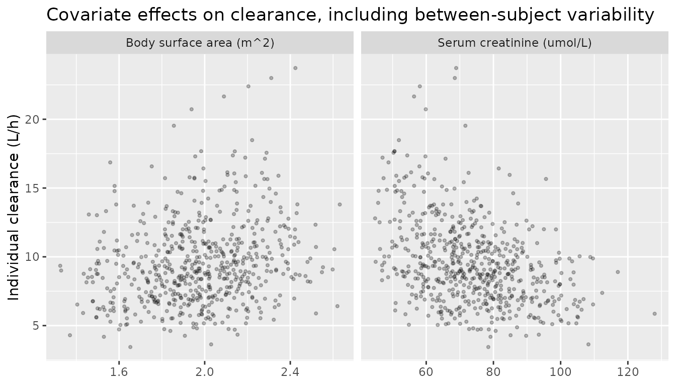

Comparison against the reported concentrations

Blackman 2026 reports no non-compartmental analysis, so there is no published Cmax / AUC / half-life table to compare against. What it does report (Table 1) is the distribution of the first, second and third measured concentrations, drawn at approximately 24, 48 and 72 h. Those are the quantities compared below.

observed <- tibble::tribble(
  ~nominal_time, ~label,            ~obs_median, ~obs_min, ~obs_max,
  24,            "1st concentration", 4.21,        0.16,     108.04,
  48,            "2nd concentration", 0.12,        0.02,       5.28,
  72,            "3rd concentration", 0.05,        0.02,       3.13
)

sim_key <- sim |>
  dplyr::filter(time %in% c(24, 48, 72)) |>
  dplyr::group_by(arm, time) |>
  dplyr::summarise(sim_median = median(Cc), .groups = "drop") |>
  tidyr::pivot_wider(names_from = arm, values_from = sim_median)

sim_key |>
  dplyr::left_join(observed, by = c("time" = "nominal_time")) |>
  dplyr::select(label, time, `2 h infusion`, `4.7 h infusion`,
                `24 h infusion`, obs_median, obs_min, obs_max) |>
  dplyr::rename(
    "Sample"                     = label,
    "Nominal time (h)"           = time,
    "Observed median (mg/L)"     = obs_median,
    "Observed min (mg/L)"        = obs_min,
    "Observed max (mg/L)"        = obs_max
  ) |>
  knitr::kable(
    digits = 3,
    caption = paste("Simulated median concentration by infusion-duration arm",
                    "against the Table 1 observed distribution (training set,",
                    "all regimens pooled).")
  )

Simulated median concentration by infusion-duration arm against the Table 1 observed distribution (training set, all regimens pooled).

Sample	Nominal time (h)	2 h infusion	4.7 h infusion	24 h infusion	Observed median (mg/L)	Observed min (mg/L)	Observed max (mg/L)
1st concentration	24	1.281	1.584	31.428	4.21	0.16	108.04
2nd concentration	48	0.147	0.187	0.489	0.12	0.02	5.28
3rd concentration	72	0.068	0.075	0.109	0.05	0.02	3.13

The 48 h and 72 h medians agree closely with the observed values at the median short infusion. The 24 h concentration is the one that moves most with infusion duration – roughly 25-fold across the arms – so the pooled observed median of 4.21 mg/L is expected to fall between the short and long arms rather than to match any one of them. That is the check applied here.

med_at <- function(arm_label, tt) {
  v <- sim$Cc[sim$arm == arm_label & sim$time == tt]
  stopifnot(length(v) == n_arm)   # a zero-row lookup would make every check below vacuous
  median(v)
}

c24_short <- med_at("4.7 h infusion", 24)
c24_long  <- med_at("24 h infusion",  24)
c48_short <- med_at("4.7 h infusion", 48)
c72_short <- med_at("4.7 h infusion", 72)

cat(sprintf("C24 short = %.2f, C24 long = %.2f, observed pooled median = 4.21 mg/L\n",
            c24_short, c24_long))
#> C24 short = 1.58, C24 long = 31.43, observed pooled median = 4.21 mg/L
cat(sprintf("C48 short = %.4f (observed 0.12), C72 short = %.4f (observed 0.05) mg/L\n",
            c48_short, c72_short))
#> C48 short = 0.1875 (observed 0.12), C72 short = 0.0748 (observed 0.05) mg/L

stopifnot(
  # The pooled observed 24 h median is bracketed by the short and long arms.
  # Realised 1.3-1.6 (short) and 27-33 (long) across renders; the bracket has
  # an order of magnitude of headroom on each side, and still fails if a
  # mis-transcribed CL, volume or dose moves the profile several-fold.
  c24_short < 4.21, c24_long > 4.21,
  # Structural agreement at 48 and 72 h, where the observed median is not
  # regimen-sensitive. A factor-of-three band around the observed value; a
  # transcription error in CL or a volume moves these by far more.
  c48_short > 0.12 / 3, c48_short < 0.12 * 3,
  c72_short > 0.05 / 3, c72_short < 0.05 * 3
)

PKNCA validation

sim_nca <- sim |>
  dplyr::filter(!is.na(Cc)) |>
  dplyr::select(id, time, Cc, arm)

# Guarantee a time = 0 row per subject. For an IV infusion the pre-dose
# concentration is 0; existing time = 0 rows win via .keep_all on the first
# occurrence.
sim_nca <- dplyr::bind_rows(
  sim_nca,
  sim_nca |> dplyr::distinct(id, arm) |> dplyr::mutate(time = 0, Cc = 0)
) |>
  dplyr::distinct(id, arm, time, .keep_all = TRUE) |>
  dplyr::arrange(id, arm, time)

dose_df <- events |>
  dplyr::filter(evid == 1) |>
  dplyr::select(id, time, amt, arm, dur)

conc_obj <- PKNCA::PKNCAconc(sim_nca, Cc ~ time | arm + id,
                             concu = "mg/L", timeu = "h")
dose_obj <- PKNCA::PKNCAdose(dose_df, amt ~ time | arm + id,
                             doseu = "mg", route = "intravascular",
                             duration = "dur")

intervals <- data.frame(
  start      = 0,
  end        = Inf,
  cmax       = TRUE,
  tmax       = TRUE,
  auclast    = TRUE,
  aucinf.obs = TRUE,
  half.life  = TRUE,
  cl.obs     = TRUE
)

nca_res <- PKNCA::pk.nca(PKNCA::PKNCAdata(conc_obj, dose_obj, intervals = intervals))

nca_tbl <- as.data.frame(nca_res$result) |>
  dplyr::filter(PPTESTCD %in% c("cmax", "tmax", "auclast", "aucinf.obs",
                                "half.life", "cl.obs")) |>
  dplyr::group_by(arm, PPTESTCD) |>
  dplyr::summarise(median = median(PPORRES, na.rm = TRUE), .groups = "drop") |>
  tidyr::pivot_wider(names_from = PPTESTCD, values_from = median)

nca_tbl |>
  dplyr::select(arm, cmax, tmax, auclast, aucinf.obs, half.life, cl.obs) |>
  dplyr::rename(
    "Infusion arm"        = arm,
    "Cmax (mg/L)"         = cmax,
    "Tmax (h)"            = tmax,
    "AUClast (mg*h/L)"    = auclast,
    "AUC0-inf (mg*h/L)"   = aucinf.obs,
    "t1/2 (h)"            = half.life,
    "CL (L/h)"            = cl.obs
  ) |>
  knitr::kable(digits = 2,
               caption = "Median NCA parameters by infusion arm (simulated cohort).")

Median NCA parameters by infusion arm (simulated cohort).

Infusion arm	Cmax (mg/L)	Tmax (h)	AUClast (mg*h/L)	AUC0-inf (mg*h/L)	t1/2 (h)	CL (L/h)
2 h infusion	159.79	2.00	735.83	737.73	41.11	9.12
24 h infusion	31.43	24.00	769.58	773.36	32.70	8.96
4.7 h infusion	110.80	4.75	777.22	780.17	42.56	9.10

NCA clearance against the model’s structural clearance

The paper publishes no NCA, but the NCA-derived clearance is a strong internal identity check: CL = dose / AUC0-inf must recover the structural clearance the model was given, subject to the extrapolation error of a 53 h terminal phase sampled to 96 h. cl.obs is returned in dose-over-concentration units (mg / (mg/L * h)) which for this model is L/h directly.

cl_struct <- sim |>
  dplyr::distinct(id, .keep_all = TRUE) |>
  dplyr::select(id, arm, cl)

cl_cmp <- as.data.frame(nca_res$result) |>
  dplyr::filter(PPTESTCD == "cl.obs") |>
  dplyr::select(id, arm, cl_nca = PPORRES) |>
  # 1:1 join on the per-subject NCA result table -- not a per-time-point join.
  dplyr::left_join(cl_struct, by = c("id", "arm")) |>
  dplyr::mutate(pct_diff = 100 * (cl_nca - cl) / cl)

stopifnot(nrow(cl_cmp) == 3L * n_arm, !anyNA(cl_cmp$pct_diff))

cl_cmp |>
  dplyr::group_by(arm) |>
  dplyr::summarise(
    `Median structural CL (L/h)` = median(cl),
    `Median NCA CL (L/h)`        = median(cl_nca),
    `Median % difference`        = median(pct_diff),
    `90th pctile |% difference|` = quantile(abs(pct_diff), 0.90),
    .groups = "drop"
  ) |>
  dplyr::rename("Infusion arm" = arm) |>
  knitr::kable(digits = 2,
               caption = "NCA-derived clearance against the model's structural clearance.")

NCA-derived clearance against the model’s structural clearance.

Infusion arm	Median structural CL (L/h)	Median NCA CL (L/h)	Median % difference	90th pctile |% difference|
2 h infusion	9.11	9.12	0.08	0.28
24 h infusion	8.94	8.96	0.06	0.38
4.7 h infusion	9.09	9.10	0.09	0.25

# Centre and robust envelope, not extremes: which subjects land in the tail of
# the AUC extrapolation is not reproducible across rxode2 builds or thread
# counts. Realised median 0.06-0.09% and 90th percentile 0.25-0.38% across the
# three arms, so the bounds below carry more than an order of magnitude of
# headroom while still failing immediately on a mis-transcribed clearance,
# volume or dose (those move the distribution by tens of percent).
stopifnot(
  abs(median(cl_cmp$pct_diff)) < 2,
  quantile(abs(cl_cmp$pct_diff), 0.90) < 5
)

# The NCA terminal half-life should recover the model's gamma-phase half-life
# (the eigenvalue computed above), within the resolution of a 96 h sampling
# window on a ~53 h terminal phase.
hl_gamma <- max(hl)
hl_nca <- as.data.frame(nca_res$result) |>
  dplyr::filter(PPTESTCD == "half.life") |>
  dplyr::pull(PPORRES)

cat(sprintf("Model gamma-phase t1/2 = %.1f h; median NCA t1/2 = %.1f h\n",
            hl_gamma, median(hl_nca, na.rm = TRUE)))
#> Model gamma-phase t1/2 = 53.3 h; median NCA t1/2 = 38.9 h

# Median only, with generous headroom: the NCA half-life is a log-linear
# regression over whatever terminal points each subject's profile offers, and
# a 96 h window on a three-phase profile does not fully resolve the gamma
# phase. It therefore reads BELOW the eigenvalue value (realised median ~39 h
# against a gamma-phase 53.3 h) -- expected, not a discrepancy.
stopifnot(median(hl_nca, na.rm = TRUE) > 25, median(hl_nca, na.rm = TRUE) < 70)

What these two checks do and do not establish: they confirm that the ODE system, the infusion handling and the sampling grid are mutually consistent, and that AUC extrapolation past 96 h is negligible (AUClast and AUC0-inf differ by well under 1%). They are internal-consistency checks, not an independent confirmation of the parameter transcription – the paper reports no NCA to compare against. The transcription itself is checked by the deterministic closed-form and covariate-equation tests above, by the concentration comparison against Table 1, and line by line by the source-trace table.

Assumptions and deviations

• Training set, not the full cohort. population$n_subjects is 145, the training subset the model was fit to, not the 208-patient cohort described in Table 1. Table 1’s training column is used for every demographic figure.
• Only the final model is packaged. Table 2’s base and BSA-adjusted columns are development stages and are not extracted.
• The ten comparator models are not extracted from this paper. Table 3 records their structure but not their parameter values; they belong to their own publications. Taylor_2020_methotrexate and Olivo_2024_methotrexate are independently available in nlmixr2lib.
• Random-effect scale inferred, not stated. Table 2 labels the variability rows %CV without declaring SD vs variance. The SD reading is established above by three independent checks and the model file squares the entries.
• Four IOV occasions. The paper reports one inter-occasion variance on clearance shared across all occasions and does not fix an occasion count (patients contributed a median of 3 cycles, range 1-12). Four occasions are encoded following the registered Jonsson_2011_ethambutol idiom; because the variance is common to every occasion, extending the chain is a mechanical copy of the fix() lines. The vignette simulates a single occasion (OCC = 1).
• Covariate distributions are simulated. Individual data are not public (IRB / consent restriction). BSA and serum creatinine are drawn from truncated normals matched to the Table 1 training-set mean, SD and range, and sex from a 60% female Bernoulli. Correlation between BSA, creatinine and sex is not modelled – the paper reports no joint distribution.
• Dose and regimen. The cohort simulates the Table 1 median dose of 3.5 g/m^2 across three infusion durations spanning the reported 2.0-27.9 h range. The paper’s loading-dose-plus-maintenance regimen (22% of infusions) is not separately simulated.
• Leucovorin is not represented. All patients received leucovorin rescue from 24 h; it is not part of the published model.
• No published NCA to compare against. The paper reports predictive-performance metrics (RMSE, MPE, MAPE, F20, F30) computed against its own held-out test set rather than NCA parameters. The PKNCA section therefore validates the model against itself (NCA clearance vs structural clearance, NCA half-life vs the eigenvalue half-life) and against the Table 1 observed concentration distribution.
• All parameter values are from the paper’s tables and text. No value was digitised from a figure, obtained by correspondence, or carried from another publication.

Errata and internal inconsistencies in the source

Three inconsistencies were found in the published paper. All are transcribed as printed; none is silently corrected.

1. The sex effect is negligible yet is reported as a substantial improvement in fit. Table 2 gives theta9 = 0.01 (SE 0.05), 95% CI [-0.08, 0.11], so female clearance is 1.0% above male and the interval comfortably spans zero. Yet the Results state that adding sex to the SCR model took the OFV reduction from 119.19 to 144.91, and the Discussion describes “a substantial reduction in OFV (25.7 units)”. A parameter whose CI includes zero cannot plausibly carry a 25.7-unit drop in objective function. The estimate and its standard error are mutually consistent (0.01 +/- 1.96 * 0.05 = [-0.088, 0.108], matching the printed CI), and the OFV values are internally consistent with each other (-2512.1 - (-2367.2) = 144.9), so both halves of the paper are self-consistent and mutually contradictory. The printed point estimate is used, and the resulting sex effect on simulated profiles is negligible.

2. The theta8 confidence interval is printed upper-bound-first. Table 2 shows -0.56 (0.08) [-0.42, -0.74]. The Wald interval is -0.56 +/- 1.96 * 0.08 = [-0.717, -0.403], so the printed bounds are correct but in reverse order. No value is affected.

3. The Table 3 footnote transposes Q3 and V3. It reads “Q3, volume of distribution in the second peripheral compartment; V3, intercompartmental clearance…”. The Table 2 footnote has them the right way round (“Q3, intercompartmental clearance between the main compartment and the secondary peripheral compartment (L/hour); V3, and volume of distribution in the secondary peripheral compartment (L)”), and the units in Table 2 (Q3 = 0.14 L/h, V3 = 10.60 L) confirm the Table 2 reading. The model follows Table 2.

Additionally, the serum-creatinine centering constant in the Table 2 equation is 68.08 umol/L, close to but not identical with the Table 1 training-set median of 68.5 umol/L (overall cohort median 68.1). Serum creatinine was a time-varying covariate, so the model’s constant is a per-record median rather than a per-subject one. The BSA centering constant of 1.97 m^2 matches the Table 1 median exactly.

No erratum or corrigendum for this article was located.