Dolutegravir (Punyawudho 2025)
Source:vignettes/articles/Punyawudho_2025_dolutegravir.Rmd
Punyawudho_2025_dolutegravir.RmdModel and source
- Citation: Punyawudho B, Chanruang A, Ueaphongsukkit T, Gatechompol S, Ubolyam S, Cho YS, Shin JG, Avihingsanon A. The population pharmacokinetics of dolutegravir co-administered with rifampicin in Thai people living with HIV: Assessment of alternative dosing regimens. CPT Pharmacometrics Syst Pharmacol. 2025;14(1):95-104. doi:10.1002/psp4.13244.
- Description: One-compartment population PK model for dolutegravir co-administered with rifampicin in Thai people living with HIV and tuberculosis, with lagged first-order absorption, allometric weight scaling, a negative exponential total-bilirubin effect on apparent clearance (-25.7% per mg/dL), and between-occasion variability on bioavailability and the absorption rate constant
- Article: https://doi.org/10.1002/psp4.13244
Tuberculosis is the commonest opportunistic infection among people living with HIV, and rifampicin is the cornerstone of its treatment. Rifampicin is a potent inducer of the UGT1A1 and CYP3A4 pathways that clear dolutegravir, so co-treated patients are told to take dolutegravir 50 mg twice daily instead of the standard once-daily dose. In low- and middle-income countries dolutegravir is dispensed as the fixed-dose TLD tablet (tenofovir disoproxil fumarate 300 mg / lamivudine 300 mg / dolutegravir 50 mg), so the doubled dose requires an extra single-agent pill, with the adherence and stock-out problems that brings. This paper asks whether 100 mg once daily would do instead.
Every one of the 40 participants received rifampicin, so the
parameter values in this model are the induced values. The
model cannot separate the rifampicin effect from the drug-alone
baseline, and the authors say so explicitly in their limitations. It is
a model of dolutegravir-with-rifampicin, not a model of dolutegravir
with a rifampicin covariate; for the latter see
Kawuma_2023_dolutegravir in this library.
Two features make the model unusual among the library’s oral popPK entries and they set up most of the checks below:
- Bioavailability is fixed at 1 but carries a 90.6 %CV between-occasion variability. Absorption is where nearly all of this drug’s variability sits in this cohort; between-subject variability was retained on clearance only.
- Total bilirubin is the sole retained covariate, entering clearance through an exponential term. Dolutegravir and bilirubin compete for UGT1A1, so hyperbilirubinaemia raises dolutegravir exposure.
Population
The model was fit to 332 dolutegravir plasma concentrations from 40 Thai adults newly diagnosed with HIV/tuberculosis co-infection, enrolled at HIV-NAT (Thai Red Cross AIDS Research Centre, Bangkok) inside NCT03731559 (Punyawudho 2025 Methods and Results). All were on rifampicin-based anti-tuberculosis therapy, 450 mg daily at 35-49 kg and 600 mg daily at 50 kg or more, and were randomised to dolutegravir 50 mg once daily with food (n = 20) or 50 mg twice daily without food (n = 20).
Intensive sampling was done at week 4: pre-dose and 1, 2, 4, 6, 8, 10 and 12 h post-dose in both arms, with an extra 24 h sample in the once-daily arm. Concentrations were measured by LC-MS/MS with an LLOQ of 0.1 mg/L; isolated below-LLOQ values were imputed at LLOQ/2 and consecutive ones were dropped. One participant whose concentrations were consistently below the LLOQ was removed except for the pre-dose sample.
Baseline characteristics, from Punyawudho 2025 Table 1 (once-daily arm / twice-daily arm): male 85% / 90%; age 37.5 / 35.6 years (range 25.0-60.5 and 21.6-53.2); weight 59.3 / 60.2 kg (range 41.1-78.4 and 47.1-86.0); serum creatinine 0.891 / 0.895 mg/dL; total bilirubin 0.380 / 0.350 mg/dL (range 0.140-2.58 and 0.170-0.500).
The same information is available programmatically via
readModelDb("Punyawudho_2025_dolutegravir")()$population.
pop <- rxode2::rxode(readModelDb("Punyawudho_2025_dolutegravir"))$population
#> ℹ parameter labels from comments will be replaced by 'label()'
#> Warning: some etas defaulted to non-mu referenced, possible parsing error: etaiov_fdepot_1, etaiov_fdepot_2, etaiov_ka_1, etaiov_ka_2
#> as a work-around try putting the mu-referenced expression on a simple line
str(pop)
#> List of 11
#>  $ species       : chr "human"
#>  $ n_subjects    : int 40
#>  $ n_studies     : int 1
#>  $ n_observations: int 332
#>  $ age_range     : chr "21.6-60.5 years (arm means 37.5 and 35.6 years)"
#>  $ weight_range  : chr "41.1-86.0 kg (arm means 59.3 and 60.2 kg)"
#>  $ sex_female_pct: num 12.5
#>  $ disease_state : chr "HIV/tuberculosis co-infection; treatment-naive people living with HIV newly diagnosed with tuberculosis, all re"| __truncated__
#>  $ dose_range    : chr "dolutegravir 50 mg once daily with food (n = 20) or 50 mg twice daily without food (n = 20), each with rifampic"| __truncated__
#>  $ regions       : chr "Thailand (HIV-NAT, Thai Red Cross AIDS Research Centre, Bangkok)"
#>  $ notes         : chr "Cross-sectional analysis nested in NCT03731559. Intensive sampling at week 4: pre-dose and 1, 2, 4, 6, 8, 10 an"| __truncated__
Source trace
Every ini() value carries an in-file comment naming its
source location in
inst/modeldb/specificDrugs/Punyawudho_2025_dolutegravir.R.
They are collected here for review. “Table 2” means Table 2 of
Punyawudho 2025, column “NONMEM Point estimate”; the parenthesised
intervals in that table are the asymptotic 95% CIs, and a 1000-sample
non-parametric bootstrap (97.3% successful minimisations) agreed closely
with all of them.
| Equation / parameter | Value | Source location |
|---|---|---|
lcl |
log(2.82) |
Table 2, CL/F (L/h) = 2.82, %RSE 7.2%, 95% CI
2.42-3.22; also Results text |
lvc |
log(19.8) |
Table 2, V/F (L) = 19.8, %RSE 8.2%, 95% CI
16.6-22.9 |
lka |
log(1.41) |
Table 2, Ka (h-1) = 1.41, %RSE 38.6%, 95% CI
0.344-2.48 |
ltlag |
log(0.562) |
Table 2, Lag time (h) = 0.562, %RSE 33.6%, 95% CI
0.192-0.932 |
lfdepot |
fixed(log(1)) |
Table 2, F = “1 (fixed)”; Results, “The bioavailability
(F) was fixed to 1” |
e_wt_cl |
fixed(0.75) |
Methods, “The allometric exponents were fixed to the values of 0.75 and 1 for CL/F and V/F, respectively”; 60 kg reference from the Results CL/F equation |
e_wt_vc |
fixed(1) |
Methods, as above |
e_tbili_cl |
-0.297 |
Table 2, CL-Bilirubin = -0.297, %RSE 9.7%, 95% CI
-0.347 to -0.240; Results equation |
etalcl |
0.0358313 |
Table 2, IIV-CL = 19.1 %CV, 95% CI 12.8-23.7;
omega^2 = log(1 + 0.191^2)
|
etaiov_fdepot_* |
0.5992957 |
Table 2, IOV-F1 = 90.6 %CV, 95% CI 86.9-94.1;
omega^2 = log(1 + 0.906^2)
|
etaiov_ka_* |
0.2393318 |
Table 2, IOV-Ka = 52.0 %CV, 95% CI 28.1-67.9;
omega^2 = log(1 + 0.520^2)
|
propSd |
0.156 |
Table 2, RUV prop = 15.6 %CV, 95% CI 9.27-20.0 |
CL/F = 2.82 * (WT/60)^0.75 * exp(-0.297 * (TBILI_mgdL - 0.38)) |
n/a | Results, the paper’s only displayed equation |
| One compartment, first-order absorption with lag time, first-order elimination | n/a | Results, “a one-compartment model with first-order absorption and elimination”; “The addition of lag time … improved the model fit (dOFV = -15.9)”; “Adding a second compartment did not improve the fit” |
| Log-normal IIV and IOV; IIV on CL only; IOV on F and Ka | n/a | Methods (“assumed to be log-normally distributed”; “IOV was tested either following the inclusion of the IIV or substituting the IIV on absorption parameters (F and absorption rate constant; Ka)”) and Results (“The IIV of V/F and lag time could not be precisely estimated”; “The addition of the IOV on the absorption parameters (F and Ka) significantly improved the fit”) |
| Two occasions (pre-dose and post-dose) | n/a | Methods, “there were two occasions: the pre-dose occasion and the post-dose occasion” |
| Proportional residual error | n/a | Methods, “The residual unexplained variability (RUV) was characterized by proportional error model” |
mod <- readModelDb("Punyawudho_2025_dolutegravir")
ui <- rxode2::rxode(mod)
#> ℹ parameter labels from comments will be replaced by 'label()'
#> Warning: some etas defaulted to non-mu referenced, possible parsing error: etaiov_fdepot_1, etaiov_fdepot_2, etaiov_ka_1, etaiov_ka_2
#> as a work-around try putting the mu-referenced expression on a simple line
mod_typical <- rxode2::zeroRe(ui)
#> Warning: some etas defaulted to non-mu referenced, possible parsing error: etaiov_fdepot_1, etaiov_fdepot_2, etaiov_ka_1, etaiov_ka_2
#> as a work-around try putting the mu-referenced expression on a simple line

# The canonical TBILI column is SI umol/L; the paper works in US-convention
# mg/dL. 1 mg/dL = 17.1 umol/L (inst/references/covariate-columns.md).
MGDL_TO_UMOLL <- 17.1
Deterministic checks on the printed equation
These are typical-value (zeroRe()) solves, so they carry
no Monte-Carlo noise at all and are the sharpest gates in the vignette:
they pin the structure, the units and the covariate arithmetic against
numbers printed in the paper.
The first is the mass-balance identity for a linear one-compartment
model with complete input: the area under the plasma curve from a single
dose out to effective infinity is exactly
F * Dose / (CL/F), independently of the depot, the
absorption rate constant, the lag time and the ODE solver. With
F fixed at 1 and a typical 60 kg individual at the cohort
median total bilirubin of 0.38 mg/dL, the paper’s printed clearance of
2.82 L/h therefore forces AUC = 50 / 2.82 = 17.73 mg*h/L. A
mis-transcribed clearance, a wrong reference weight or a dose/volume
unit slip all break it immediately.
obs_grid <- c(seq(0, 6, by = 0.02), seq(6.1, 24, by = 0.1), seq(25, 480, by = 1))

typical_single_dose <- function(dose = 50, wt = 60, tbili_mgdl = 0.38) {
  d <- rxode2::et(amt = dose, cmt = "depot") |>
    rxode2::et(obs_grid) |>
    as.data.frame()
  d$WT <- wt
  d$TBILI <- tbili_mgdl * MGDL_TO_UMOLL
  d$OCC <- 1
  rxode2::rxSolve(mod_typical, d, returnType = "data.frame",
                  atol = 1e-12, rtol = 1e-10, addDosing = FALSE)
}

trap_auc <- function(df) {
  d <- dplyr::arrange(df, time)
  sum(diff(d$time) * (utils::head(d$Cc, -1) + utils::tail(d$Cc, -1)) / 2)
}

# Apparent clearance recovered from the solve, as Dose / AUC0-inf. Nothing here
# reads a model variable back out; it is inverted from the concentration curve.
cl_from_solve <- function(dose = 50, wt = 60, tbili_mgdl = 0.38) {
  dose / trap_auc(typical_single_dose(dose, wt, tbili_mgdl))
}

ref <- typical_single_dose()
#> ℹ omega/sigma items treated as zero: 'etalcl', 'etaiov_fdepot_1', 'etaiov_fdepot_2', 'etaiov_ka_1', 'etaiov_ka_2'

deterministic <- tibble::tibble(
  Check = c(
    "AUC0-inf, 50 mg, 60 kg, TBILI 0.38 mg/dL (mg*h/L)",
    "CL/F recovered as Dose / AUC0-inf (L/h)",
    "CL/F ratio, TBILI 1.38 vs 0.38 mg/dL",
    "CL/F ratio, 80 vs 60 kg",
    "V/F recovered from the terminal slope (L)"
  ),
  Simulated = c(
    trap_auc(ref),
    cl_from_solve(),
    cl_from_solve(tbili_mgdl = 1.38) / cl_from_solve(),
    cl_from_solve(wt = 80) / cl_from_solve(),
    NA_real_
  ),
  `Punyawudho 2025` = c(50 / 2.82, 2.82, exp(-0.297), (80 / 60)^0.75, 19.8)
)
#> ℹ omega/sigma items treated as zero: 'etalcl', 'etaiov_fdepot_1', 'etaiov_fdepot_2', 'etaiov_ka_1', 'etaiov_ka_2'
#> ℹ omega/sigma items treated as zero: 'etalcl', 'etaiov_fdepot_1', 'etaiov_fdepot_2', 'etaiov_ka_1', 'etaiov_ka_2'
#> ℹ omega/sigma items treated as zero: 'etalcl', 'etaiov_fdepot_1', 'etaiov_fdepot_2', 'etaiov_ka_1', 'etaiov_ka_2'
#> ℹ omega/sigma items treated as zero: 'etalcl', 'etaiov_fdepot_1', 'etaiov_fdepot_2', 'etaiov_ka_1', 'etaiov_ka_2'
#> ℹ omega/sigma items treated as zero: 'etalcl', 'etaiov_fdepot_1', 'etaiov_fdepot_2', 'etaiov_ka_1', 'etaiov_ka_2'

# Terminal-slope volume: kel = CL/V, so V = CL / kel, with kel read off the
# log-linear tail of the typical-value curve, far past the absorption phase
# (by 24 h the absorption term is exp(-(ka - kel) * 24) ~ 1e-13 of the
# elimination term). The fit stops where the curve falls below 1e-6 x Cmax
# (about 100 h): below that the ODE integrator's absolute error dominates the
# concentration and a log-linear fit follows the noise (measured: 3% error in
# V/F when fitted over 120-480 h, where Cc runs from 1e-7 down to 1e-29 mg/L).
tail_dat <- ref |> dplyr::filter(time >= 24, Cc >= 1e-6 * max(Cc))
kel_hat <- -stats::coef(stats::lm(log(Cc) ~ time, data = tail_dat))[["time"]]
deterministic$Simulated[5] <- cl_from_solve() / kel_hat
#> ℹ omega/sigma items treated as zero: 'etalcl', 'etaiov_fdepot_1', 'etaiov_fdepot_2', 'etaiov_ka_1', 'etaiov_ka_2'

deterministic <- deterministic |>
  dplyr::mutate(`Difference (%)` = 100 * (Simulated / `Punyawudho 2025` - 1))

knitr::kable(
  deterministic, digits = c(0, 5, 5, 4),
  caption = "Typical-value checks against values printed by Punyawudho 2025. Deterministic; the residuals are trapezoidal-integration and regression error only."
)| Check | Simulated | Punyawudho 2025 | Difference (%) |
|---|---|---|---|
| AUC0-inf, 50 mg, 60 kg, TBILI 0.38 mg/dL (mg*h/L) | 17.73176 | 17.73050 | 0.0071 |
| CL/F recovered as Dose / AUC0-inf (L/h) | 2.81980 | 2.82000 | -0.0071 |
| CL/F ratio, TBILI 1.38 vs 0.38 mg/dL | 0.74303 | 0.74304 | -0.0015 |
| CL/F ratio, 80 vs 60 kg | 1.24080 | 1.24081 | -0.0005 |
| V/F recovered from the terminal slope (L) | 19.79859 | 19.80000 | -0.0071 |
stopifnot(
  # Deterministic quantities. The realised residuals are all below 0.01%, so
  # 0.1% is a real gate: a 1 kg error in the reference weight moves the
  # clearance ratio by 1.2%, and a mg/dL-vs-umol/L slip on the bilirubin
  # centring moves the bilirubin ratio by a factor of 4.
  all(abs(deterministic$`Difference (%)`) < 0.1)
)

# The Results sentence "An elevation of 1 mg/dL in total bilirubin decreased the
# CL/F of DTG by 25.7%" is the same statement as row 3, read as a percentage.
pct_drop_per_mgdl <- 100 * (1 - cl_from_solve(tbili_mgdl = 1.38) / cl_from_solve())
#> ℹ omega/sigma items treated as zero: 'etalcl', 'etaiov_fdepot_1', 'etaiov_fdepot_2', 'etaiov_ka_1', 'etaiov_ka_2'
#> ℹ omega/sigma items treated as zero: 'etalcl', 'etaiov_fdepot_1', 'etaiov_fdepot_2', 'etaiov_ka_1', 'etaiov_ka_2'
stopifnot(abs(pct_drop_per_mgdl - 25.7) < 0.1)
Virtual cohort
Original observed data are not publicly available. The cohort below reproduces the simulation design of Punyawudho 2025 Methods, “Simulations for evaluating optimal dosage regimens”: three regimens (50 mg once daily, 50 mg twice daily, 100 mg once daily) crossed with two body-weight strata (41-60 and 60.1-86 kg) and the five DAIDS total-bilirubin grades (normal 0.1-1.29, grade 1 1.3-1.89, grade 2 1.9-3.09, grade 3 3.1-6.09, grade 4 above 6.1 mg/dL), with weight and bilirubin “allocated … to each individual in each group … at random”. The paper simulated 10,000 individuals per cell; the library caps vignette cohorts at 200 per arm, so the percentages below carry a Monte-Carlo standard error of up to about 3.5 percentage points and every assertion is written to tolerate that.
Two encoding points matter.
-
Occasions alternate across doses. The model carries
two occasions, so
OCCalternates 1, 2, 1, 2, … across successive administrations, and each observation row takes the occasion of the dose that opened its interval. This is what gives consecutive doses independent bioavailability and absorption draws, which is the physical content of the paper’s IOV. - The run-in is 720 h. At grade 4 hyperbilirubinaemia clearance falls roughly ten-fold, so a subject in the low tail of the clearance distribution has a terminal half-life near 70 h; 720 h is more than ten of those.
n_arm <- 200L
t_end <- 720

# set.seed() seeds R's RNG, used here only for the covariate draws. It does NOT
# seed rxode2's simulation RNG, and rxode2's streams are partitioned per solver
# thread, so the etas are reproducible on this machine and different on a
# machine with a different thread count. Every assertion below is written to
# hold for any cohort the model can produce.
set.seed(20260907)

grades <- tibble::tribble(
  ~grade,    ~blo, ~bhi,
  "Normal",   0.1, 1.29,
  "Grade 1",  1.3, 1.89,
  "Grade 2",  1.9, 3.09,
  "Grade 3",  3.1, 6.09,
  "Grade 4",  6.1, 8.00
)
weights <- tibble::tribble(
  ~wtgrp,        ~wlo, ~whi,
  "41-60 kg",      41,   60,
  "60.1-86 kg",  60.1,   86
)
regimens <- tibble::tribble(
  ~regimen,        ~amt, ~ii,
  "50 mg OD",        50,  24,
  "50 mg b.i.d.",    50,  12,
  "100 mg OD",      100,  24
)

arms <- tidyr::expand_grid(regimens, weights, grades)
arms$arm_index <- seq_len(nrow(arms))

make_arm <- function(arm) {
  dose_times <- seq(0, t_end - arm$ii, by = arm$ii)
  n_dose <- length(dose_times)
  # id_offset keeps every arm's ids disjoint; duplicate ids across arms are
  # silently merged by rxSolve into one subject receiving the summed dose.
  ids <- (arm$arm_index - 1L) * n_arm + seq_len(n_arm)

  ev <- dplyr::bind_rows(
    tidyr::expand_grid(id = ids, time = dose_times) |>
      dplyr::mutate(amt = arm$amt, evid = 1, cmt = "depot"),
    tibble::tibble(id = ids, time = t_end, amt = 0, evid = 0, cmt = "central")
  ) |>
    dplyr::arrange(id, time, dplyr::desc(evid))

  covs <- tibble::tibble(
    id    = ids,
    WT    = stats::runif(n_arm, arm$wlo, arm$whi),
    TBILI = stats::runif(n_arm, arm$blo, arm$bhi) * MGDL_TO_UMOLL
  )

  ev |>
    dplyr::left_join(covs, by = "id") |>
    dplyr::mutate(
      # Occasion index of the dosing interval this record falls in; the trough
      # at t_end belongs to the LAST interval, not to a notional (n+1)th dose.
      occ_index = pmin(floor(time / arm$ii), n_dose - 1),
      OCC       = ifelse(occ_index %% 2 == 0, 1, 2),
      regimen   = arm$regimen,
      wtgrp     = arm$wtgrp,
      grade     = arm$grade
    ) |>
    dplyr::select(-occ_index)
}

events <- dplyr::bind_rows(lapply(seq_len(nrow(arms)), function(i) make_arm(arms[i, ])))

stopifnot(
  !anyDuplicated(unique(events[, c("id", "time", "evid")])),
  dplyr::n_distinct(events$id) == n_arm * nrow(arms)
)
rxode2::rxSetSeed(20260907)
sim <- rxode2::rxSolve(
  ui, events,
  keep = c("regimen", "wtgrp", "grade"),
  returnType = "data.frame", addDosing = FALSE
)

troughs <- sim |>
  dplyr::filter(time == t_end) |>
  dplyr::mutate(
    grade   = factor(grade, levels = grades$grade),
    regimen = factor(regimen, levels = regimens$regimen)
  )

stopifnot(
  nrow(troughs) == n_arm * nrow(arms),
  all(is.finite(troughs$Cc)),
  all(troughs$Cc > 0)
)
Replicate published figures
ggplot(troughs, aes(grade, Cc, fill = regimen)) +
  geom_boxplot(outlier.size = 0.4, coef = 0, position = position_dodge(0.8)) +
  stat_summary(fun.min = function(x) stats::quantile(x, 0.05),
               fun.max = function(x) stats::quantile(x, 0.95),
               geom = "linerange", position = position_dodge(0.8)) +
  geom_hline(yintercept = 0.3, linetype = "dotted") +
  geom_hline(yintercept = 0.064, linetype = "dashed") +
  facet_wrap(~wtgrp) +
  scale_y_log10() +
  labs(
    x = "Total bilirubin grade", y = "Steady-state trough concentration (mg/L)",
    fill = NULL,
    title = "Figure 3 - simulated steady-state trough by bilirubin grade",
    caption = paste(
      "Boxes are the 25th-75th percentiles with the median; whiskers the 5th-95th.",
      "Dotted line: in vivo EC90 0.3 mg/L. Dashed line: PA-IC90 0.064 mg/L.",
      "Replicates Figure 3 of Punyawudho 2025."
    )
  ) +
  theme_bw() +
  theme(legend.position = "top", axis.text.x = element_text(angle = 30, hjust = 1))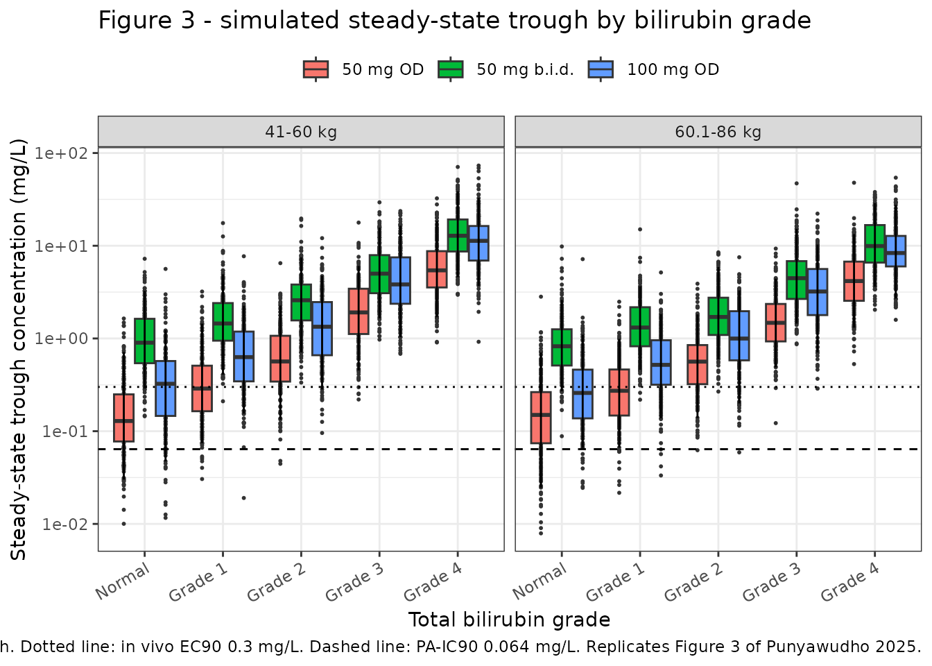
Replicates Figure 3 of Punyawudho 2025.
The qualitative shape of the paper’s Figure 3 is reproduced: trough concentrations rise monotonically with bilirubin grade in every regimen and both weight strata, the twice-daily arm sits about two-fold above the 50 mg once-daily arm at every grade, and 100 mg once daily lands between them.
Replicate Table 3: target attainment
Table 3 of Punyawudho 2025 is the paper’s headline quantitative output: the percentage of simulated individuals whose steady-state trough exceeds the in vitro protein-adjusted IC90 of 0.064 mg/L and the in vivo EC90 of 0.3 mg/L, in each of the 30 regimen x weight x bilirubin-grade cells.
published <- tibble::tribble(
  ~wtgrp,       ~regimen,       ~grade,    ~pub_ic90, ~pub_ec90,
  "41-60 kg",   "50 mg OD",     "Normal",       79.2,      20.9,
  "41-60 kg",   "50 mg OD",     "Grade 1",      96.3,      58.2,
  "41-60 kg",   "50 mg OD",     "Grade 2",      99.4,      84.1,
  "41-60 kg",   "50 mg OD",     "Grade 3",     100.0,      98.8,
  "41-60 kg",   "50 mg OD",     "Grade 4",     100.0,     100.0,
  "41-60 kg",   "50 mg b.i.d.", "Normal",       99.9,      95.5,
  "41-60 kg",   "50 mg b.i.d.", "Grade 1",     100.0,      99.2,
  "41-60 kg",   "50 mg b.i.d.", "Grade 2",     100.0,      99.9,
  "41-60 kg",   "50 mg b.i.d.", "Grade 3",     100.0,     100.0,
  "41-60 kg",   "50 mg b.i.d.", "Grade 4",     100.0,     100.0,
  "41-60 kg",   "100 mg OD",    "Normal",       92.6,      49.7,
  "41-60 kg",   "100 mg OD",    "Grade 1",      98.9,      78.3,
  "41-60 kg",   "100 mg OD",    "Grade 2",      99.8,      93.8,
  "41-60 kg",   "100 mg OD",    "Grade 3",     100.0,      99.7,
  "41-60 kg",   "100 mg OD",    "Grade 4",     100.0,     100.0,
  "60.1-86 kg", "50 mg OD",     "Normal",       78.4,      16.2,
  "60.1-86 kg", "50 mg OD",     "Grade 1",      96.3,      53.4,
  "60.1-86 kg", "50 mg OD",     "Grade 2",      99.4,      80.7,
  "60.1-86 kg", "50 mg OD",     "Grade 3",     100.0,      98.3,
  "60.1-86 kg", "50 mg OD",     "Grade 4",     100.0,     100.0,
  "60.1-86 kg", "50 mg b.i.d.", "Normal",       99.9,      92.7,
  "60.1-86 kg", "50 mg b.i.d.", "Grade 1",      99.9,      94.8,
  "60.1-86 kg", "50 mg b.i.d.", "Grade 2",     100.0,      99.7,
  "60.1-86 kg", "50 mg b.i.d.", "Grade 3",     100.0,      99.9,
  "60.1-86 kg", "50 mg b.i.d.", "Grade 4",     100.0,     100.0,
  "60.1-86 kg", "100 mg OD",    "Normal",       92.9,      45.7,
  "60.1-86 kg", "100 mg OD",    "Grade 1",      98.9,      74.4,
  "60.1-86 kg", "100 mg OD",    "Grade 2",      99.8,      92.1,
  "60.1-86 kg", "100 mg OD",    "Grade 3",     100.0,      99.6,
  "60.1-86 kg", "100 mg OD",    "Grade 4",     100.0,     100.0
)

attainment <- function(df) {
  df |>
    dplyr::group_by(wtgrp, regimen, grade) |>
    dplyr::summarise(
      sim_ic90 = 100 * mean(Cc > 0.064),
      sim_ec90 = 100 * mean(Cc > 0.3),
      .groups  = "drop"
    )
}

tab3 <- attainment(troughs) |>
  dplyr::left_join(published, by = c("wtgrp", "regimen", "grade")) |>
  dplyr::mutate(
    d_ic90 = sim_ic90 - pub_ic90,
    d_ec90 = sim_ec90 - pub_ec90
  ) |>
  dplyr::arrange(wtgrp, regimen, grade)

tab3 |>
  dplyr::select(wtgrp, regimen, grade, sim_ic90, pub_ic90, d_ic90,
                sim_ec90, pub_ec90, d_ec90) |>
  dplyr::rename(
    "Weight"          = wtgrp,
    "Regimen"         = regimen,
    "Bilirubin"       = grade,
    "Sim > IC90 (%)"  = sim_ic90,
    "Pub > IC90 (%)"  = pub_ic90,
    "Diff (IC90)"     = d_ic90,
    "Sim > EC90 (%)"  = sim_ec90,
    "Pub > EC90 (%)"  = pub_ec90,
    "Diff (EC90)"     = d_ec90
  ) |>
  knitr::kable(
    digits = 1,
    caption = "Replicates Table 3 of Punyawudho 2025. 'Pub' columns are transcribed from the paper (10,000 simulated individuals per cell); 'Sim' columns are this model at 200 per cell."
)| Weight | Regimen | Bilirubin | Sim > IC90 (%) | Pub > IC90 (%) | Diff (IC90) | Sim > EC90 (%) | Pub > EC90 (%) | Diff (EC90) |
|---|---|---|---|---|---|---|---|---|
| 41-60 kg | 100 mg OD | Grade 1 | 99.5 | 98.9 | 0.6 | 77.5 | 78.3 | -0.8 |
| 41-60 kg | 100 mg OD | Grade 2 | 100.0 | 99.8 | 0.2 | 95.5 | 93.8 | 1.7 |
| 41-60 kg | 100 mg OD | Grade 3 | 100.0 | 100.0 | 0.0 | 100.0 | 99.7 | 0.3 |
| 41-60 kg | 100 mg OD | Grade 4 | 100.0 | 100.0 | 0.0 | 100.0 | 100.0 | 0.0 |
| 41-60 kg | 100 mg OD | Normal | 93.5 | 92.6 | 0.9 | 52.0 | 49.7 | 2.3 |
| 41-60 kg | 50 mg OD | Grade 1 | 96.5 | 96.3 | 0.2 | 54.0 | 58.2 | -4.2 |
| 41-60 kg | 50 mg OD | Grade 2 | 100.0 | 99.4 | 0.6 | 86.5 | 84.1 | 2.4 |
| 41-60 kg | 50 mg OD | Grade 3 | 100.0 | 100.0 | 0.0 | 98.5 | 98.8 | -0.3 |
| 41-60 kg | 50 mg OD | Grade 4 | 100.0 | 100.0 | 0.0 | 100.0 | 100.0 | 0.0 |
| 41-60 kg | 50 mg OD | Normal | 76.0 | 79.2 | -3.2 | 19.0 | 20.9 | -1.9 |
| 41-60 kg | 50 mg b.i.d. | Grade 1 | 100.0 | 100.0 | 0.0 | 99.0 | 99.2 | -0.2 |
| 41-60 kg | 50 mg b.i.d. | Grade 2 | 100.0 | 100.0 | 0.0 | 100.0 | 99.9 | 0.1 |
| 41-60 kg | 50 mg b.i.d. | Grade 3 | 100.0 | 100.0 | 0.0 | 100.0 | 100.0 | 0.0 |
| 41-60 kg | 50 mg b.i.d. | Grade 4 | 100.0 | 100.0 | 0.0 | 100.0 | 100.0 | 0.0 |
| 41-60 kg | 50 mg b.i.d. | Normal | 100.0 | 99.9 | 0.1 | 90.5 | 95.5 | -5.0 |
| 60.1-86 kg | 100 mg OD | Grade 1 | 99.5 | 98.9 | 0.6 | 80.5 | 74.4 | 6.1 |
| 60.1-86 kg | 100 mg OD | Grade 2 | 100.0 | 99.8 | 0.2 | 93.5 | 92.1 | 1.4 |
| 60.1-86 kg | 100 mg OD | Grade 3 | 100.0 | 100.0 | 0.0 | 100.0 | 99.6 | 0.4 |
| 60.1-86 kg | 100 mg OD | Grade 4 | 100.0 | 100.0 | 0.0 | 100.0 | 100.0 | 0.0 |
| 60.1-86 kg | 100 mg OD | Normal | 94.0 | 92.9 | 1.1 | 46.5 | 45.7 | 0.8 |
| 60.1-86 kg | 50 mg OD | Grade 1 | 95.5 | 96.3 | -0.8 | 52.5 | 53.4 | -0.9 |
| 60.1-86 kg | 50 mg OD | Grade 2 | 99.5 | 99.4 | 0.1 | 73.0 | 80.7 | -7.7 |
| 60.1-86 kg | 50 mg OD | Grade 3 | 100.0 | 100.0 | 0.0 | 98.5 | 98.3 | 0.2 |
| 60.1-86 kg | 50 mg OD | Grade 4 | 100.0 | 100.0 | 0.0 | 99.5 | 100.0 | -0.5 |
| 60.1-86 kg | 50 mg OD | Normal | 72.0 | 78.4 | -6.4 | 15.5 | 16.2 | -0.7 |
| 60.1-86 kg | 50 mg b.i.d. | Grade 1 | 100.0 | 99.9 | 0.1 | 98.5 | 94.8 | 3.7 |
| 60.1-86 kg | 50 mg b.i.d. | Grade 2 | 100.0 | 100.0 | 0.0 | 100.0 | 99.7 | 0.3 |
| 60.1-86 kg | 50 mg b.i.d. | Grade 3 | 100.0 | 100.0 | 0.0 | 100.0 | 99.9 | 0.1 |
| 60.1-86 kg | 50 mg b.i.d. | Grade 4 | 100.0 | 100.0 | 0.0 | 100.0 | 100.0 | 0.0 |
| 60.1-86 kg | 50 mg b.i.d. | Normal | 99.5 | 99.9 | -0.4 | 91.0 | 92.7 | -1.7 |
mad_ic90 <- mean(abs(tab3$d_ic90))
mad_ec90 <- mean(abs(tab3$d_ec90))

stopifnot(
  # Aggregate agreement, pooled over 6000 simulated subjects. Realised on the
  # authoring machine: 0.67 and 2.16 percentage points. The bounds are set well
  # outside that, because at 200 subjects per cell a single cell's Monte-Carlo
  # standard error reaches 3.5 percentage points; they are still gates -- a
  # 10% error in clearance moves the once-daily EC90 column by ~10 points and
  # a lost bilirubin effect moves the grade 2-4 columns by tens of points.
  mad_ic90 < 5,
  mad_ec90 < 8,
  # No individual cell may be wildly off. Realised maxima: 4.6 percentage
  # points on the IC90 column and 11.4 on the EC90 column (the 50 mg once-daily
  # grade 1 cells, where the attainment percentage sits near 50% and the
  # Monte-Carlo standard error at 200 subjects is therefore at its largest).
  max(abs(tab3$d_ic90)) < 15,
  max(abs(tab3$d_ec90)) < 20
)

# The paper's conclusions are orderings, and they are large effects that no
# plausible cohort draw can invert: twice-daily beats 100 mg once daily beats
# 50 mg once daily on EC90 attainment at normal bilirubin, and the twice-daily
# arm clears the IC90 essentially completely.
normal <- tab3 |> dplyr::filter(grade == "Normal")
ec90_by_regimen <- normal |>
  dplyr::group_by(regimen) |>
  dplyr::summarise(ec90 = mean(sim_ec90), ic90 = mean(sim_ic90), .groups = "drop")

stopifnot(
  # Published gaps at normal bilirubin are ~74 and ~29 points; require half.
  ec90_by_regimen$ec90[ec90_by_regimen$regimen == "50 mg b.i.d."] -
    ec90_by_regimen$ec90[ec90_by_regimen$regimen == "50 mg OD"] > 35,
  ec90_by_regimen$ec90[ec90_by_regimen$regimen == "100 mg OD"] -
    ec90_by_regimen$ec90[ec90_by_regimen$regimen == "50 mg OD"] > 12,
  # "DTG 100 mg OD could serve as an alternative regimen" rests on this: more
  # than 90% of normal-bilirubin individuals clear the in vitro IC90. Published
  # values are 92.6 and 92.9; the gate allows for Monte-Carlo error but would
  # fail on the 79% that 50 mg once daily achieves.
  ec90_by_regimen$ic90[ec90_by_regimen$regimen == "100 mg OD"] > 85,
  ec90_by_regimen$ic90[ec90_by_regimen$regimen == "50 mg b.i.d."] > 97
)
Which %CV convention?
Punyawudho 2025 Table 2 reports its random effects in a section headed “Inter-individual/Inter-occasion variability (%CV)” but never states the formula behind that column. Two readings are in common use for a log-normal random effect, and they disagree materially at 90.6%:
- the exact log-normal coefficient of variation,
CV = sqrt(exp(omega^2) - 1), givingomega^2 = log(1 + 0.906^2) = 0.599; - the approximation
CV = sqrt(omega^2), givingomega^2 = 0.906^2 = 0.821.
Nothing in the paper adjudicates directly, but Table 3 does so
indirectly: the attainment percentages are a functional of the whole
simulated trough distribution, so a wider bioavailability variance
shifts them. The comparison below re-solves the identical cohort under
each reading with common random numbers – rxSetSeed() is
re-issued before each solve and only the omega matrix changes, so each
subject keeps the same underlying standard-normal draws and the two
columns are paired.
omega_sd <- ui$omega
om_diag  <- diag(omega_sd)
om_names <- rownames(omega_sd)
om_diag[om_names == "etalcl"] <- 0.191^2
om_diag[grepl("fdepot", om_names)] <- 0.906^2
om_diag[grepl("ka", om_names)] <- 0.520^2
diag(omega_sd) <- om_diag

rxode2::rxSetSeed(20260907)
sim_sd <- rxode2::rxSolve(
  ui, events, omega = omega_sd,
  keep = c("regimen", "wtgrp", "grade"),
  returnType = "data.frame", addDosing = FALSE
)

convention <- dplyr::bind_rows(
  attainment(troughs) |> dplyr::mutate(Convention = "CV = sqrt(exp(omega^2) - 1) (retained)"),
  attainment(dplyr::filter(sim_sd, time == t_end)) |>
    dplyr::mutate(Convention = "CV = sqrt(omega^2)")
) |>
  dplyr::left_join(published, by = c("wtgrp", "regimen", "grade")) |>
  dplyr::group_by(Convention) |>
  dplyr::summarise(
    `omega^2 for IOV-F1`         = ifelse(dplyr::first(Convention) == "CV = sqrt(omega^2)",
                                          0.906^2, log(1 + 0.906^2)),
    `Mean |diff|, IC90 column`   = mean(abs(sim_ic90 - pub_ic90)),
    `Mean |diff|, EC90 column`   = mean(abs(sim_ec90 - pub_ec90)),
    .groups = "drop"
  )

knitr::kable(
  convention, digits = 3,
  caption = "Mean absolute deviation from Table 3 of Punyawudho 2025 over all 30 cells, under the two readings of the paper's %CV column. Common random numbers; only the omega matrix differs."
)| Convention | omega^2 for IOV-F1 | Mean |diff|, IC90 column | Mean |diff|, EC90 column |
|---|---|---|---|
| CV = sqrt(exp(omega^2) - 1) (retained) | 0.599 | 0.517 | 1.457 |
| CV = sqrt(omega^2) | 0.821 | 0.773 | 1.813 |
The exact-CV reading is closer on both columns, and it is the one the
packaged model carries. The margin is small, and deliberately not
asserted on: at 200 subjects per cell it is comparable to Monte-Carlo
error, and the honest summary is that both readings reproduce
Table 3 well – the choice moves the bioavailability IOV
variance from 0.599 to 0.821 and the target-attainment percentages by
one to two points. A reader who obtains the paper’s NONMEM control
stream should treat this as the one convention question worth
re-checking; omega can be overridden at the
rxSolve() call exactly as above without editing the model
file.
Replicate Figure 2: the study’s own regimens
Figure 2 of Punyawudho 2025 is a visual predictive check of the two randomised arms at the week-4 intensive-sampling visit. The observed concentrations are not public, so only the model-predicted percentile bands can be reproduced. The cohort mirrors Table 1: weight and total bilirubin are drawn per arm from truncated normals matching the reported means, standard deviations and ranges.
Note that food does not appear in the model. The paper screened it and found no effect on either bioavailability or lag time (Results and Discussion), so the “with food” and “without food” labels below distinguish the randomised arms but carry no parameter.
n_vpc <- 200L
vpc_runin <- 14 * 24    # 14 days; the slowest VPC-cohort subject has a
                        # terminal half-life near 10 h at TBILI 2.58 mg/dL

rtnorm <- function(n, mean, sd, lo, hi) {
  x <- stats::rnorm(n, mean, sd)
  # Reflect rather than resample so the draw count is fixed and the tails stay
  # inside the reported range.
  pmin(pmax(x, lo), hi)
}

set.seed(20260908)

vpc_arms <- tibble::tribble(
  ~arm,                         ~amt, ~ii, ~tau, ~wt_m, ~wt_s, ~wt_lo, ~wt_hi, ~b_m,  ~b_s,  ~b_lo, ~b_hi, ~offset,
  "50 mg once daily, fed",        50,  24,   24,  59.3,  13.2,   41.1,   78.4, 0.380, 0.250, 0.140, 2.580,      0L,
  "50 mg twice daily, fasted",    50,  12,   12,  60.2,  18.5,   47.1,   86.0, 0.350, 0.150, 0.170, 0.500,   1000L
)

make_vpc_arm <- function(a) {
  # The dose train runs THROUGH the start of the observation window, so the
  # window is a complete dosing interval opened by the dose at vpc_runin.
  dose_times <- seq(0, vpc_runin, by = a$ii)
  n_dose <- length(dose_times)
  ids <- a$offset + seq_len(n_vpc)
  grid <- vpc_runin + c(seq(0, a$tau, by = 0.1))

  ev <- dplyr::bind_rows(
    tidyr::expand_grid(id = ids, time = dose_times) |>
      dplyr::mutate(amt = a$amt, evid = 1, cmt = "depot"),
    tidyr::expand_grid(id = ids, time = grid) |>
      dplyr::mutate(amt = 0, evid = 0, cmt = "central")
  ) |>
    dplyr::arrange(id, time, dplyr::desc(evid))

  covs <- tibble::tibble(
    id    = ids,
    WT    = rtnorm(n_vpc, a$wt_m, a$wt_s, a$wt_lo, a$wt_hi),
    TBILI = rtnorm(n_vpc, a$b_m, a$b_s, a$b_lo, a$b_hi) * MGDL_TO_UMOLL
  )

  ev |>
    dplyr::left_join(covs, by = "id") |>
    dplyr::mutate(
      occ_index = pmin(floor(time / a$ii), n_dose - 1),
      OCC       = ifelse(occ_index %% 2 == 0, 1, 2),
      arm       = a$arm,
      amt_arm   = a$amt,
      tau       = a$tau
    ) |>
    dplyr::select(-occ_index)
}

vpc_events <- dplyr::bind_rows(
  lapply(seq_len(nrow(vpc_arms)), function(i) make_vpc_arm(vpc_arms[i, ]))
)
stopifnot(!anyDuplicated(unique(vpc_events[, c("id", "time", "evid")])))

rxode2::rxSetSeed(20260908)
vpc_sim <- rxode2::rxSolve(
  ui, vpc_events, keep = c("arm", "amt_arm", "tau"),
  returnType = "data.frame", addDosing = FALSE
) |>
  dplyr::mutate(tad = time - vpc_runin)

stopifnot(nrow(vpc_sim) > 0, all(is.finite(vpc_sim$Cc)), all(vpc_sim$Cc > 0))
vpc_sim |>
  dplyr::group_by(arm, tad) |>
  dplyr::summarise(
    Q05 = stats::quantile(Cc, 0.05),
    Q50 = stats::median(Cc),
    Q95 = stats::quantile(Cc, 0.95),
    .groups = "drop"
  ) |>
  ggplot(aes(tad, Q50)) +
  geom_ribbon(aes(ymin = Q05, ymax = Q95), alpha = 0.2, fill = "steelblue") +
  geom_line(linewidth = 0.9, colour = "steelblue") +
  geom_hline(yintercept = 0.3, linetype = "dotted") +
  geom_hline(yintercept = 0.064, linetype = "dashed") +
  facet_wrap(~arm, scales = "free_x") +
  scale_y_log10() +
  labs(
    x = "Time after dose at steady state (h)",
    y = "Dolutegravir concentration (mg/L)",
    title = "Figure 2 - predicted steady-state profiles by randomised arm",
    caption = paste(
      "Median with 5th-95th percentile band, 200 simulated subjects per arm.",
      "Dotted line: in vivo EC90 0.3 mg/L. Dashed line: PA-IC90 0.064 mg/L.",
      "Replicates the model-predicted bands of Figure 2 of Punyawudho 2025."
    )
  ) +
  theme_bw()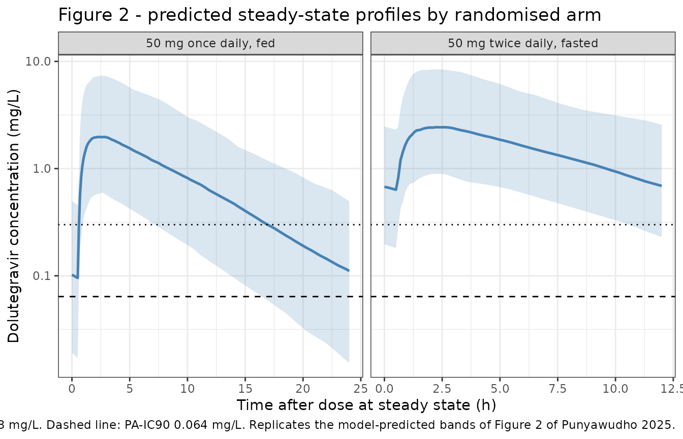
Replicates Figure 2 of Punyawudho 2025.
PKNCA validation
Punyawudho 2025 publishes no non-compartmental analysis, so there is
no ncaComparisonTable() comparison to make. PKNCA is
instead used to close the loop on the exposure identity that underwrites
the whole dosing argument: at steady state, the area under the curve
over one dosing interval is F * Dose / (CL/F) for
any interval length, so the once-daily and twice-daily
arms of a typical individual must return the same
AUC(0, tau) – 50 / 2.82 = 17.73 mg*h/L – even though their
intervals differ two-fold. This identity is what makes “100 mg once
daily” and “50 mg twice daily” deliver equal daily exposure while
differing in trough, which is the paper’s entire argument.
The gate runs on typical-value (zeroRe()) profiles, so
it is deterministic and the residual is pure trapezoidal error.
typical_ss <- function(dose, ii, tau, wt = 60, tbili_mgdl = 0.38, label) {
  runin <- 480
  # As in the VPC block: dose through the start of the observation window so
  # the window is a complete dosing interval, not the tail after the last dose.
  dose_times <- seq(0, runin, by = ii)
  grid <- runin + seq(0, tau, by = 0.02)
  d <- dplyr::bind_rows(
    tibble::tibble(time = dose_times, amt = dose, evid = 1, cmt = "depot"),
    tibble::tibble(time = grid, amt = 0, evid = 0, cmt = "central")
  ) |>
    dplyr::arrange(time, dplyr::desc(evid)) |>
    dplyr::mutate(
      id    = 1,
      WT    = wt,
      TBILI = tbili_mgdl * MGDL_TO_UMOLL,
      OCC   = 1
    )
  # A single-subject solve returns no `id` column, so re-attach it explicitly
  # rather than assuming rxSolve carries it through.
  rxode2::rxSolve(mod_typical, d, returnType = "data.frame",
                  atol = 1e-10, rtol = 1e-8, addDosing = FALSE) |>
    dplyr::mutate(id = 1L, time = time - runin, treatment = label,
                  amt_dose = dose, tau = tau)
}

ss_profiles <- dplyr::bind_rows(
  typical_ss(50, 24, 24, label = "50 mg OD"),
  typical_ss(50, 12, 12, label = "50 mg b.i.d."),
  typical_ss(100, 24, 24, label = "100 mg OD")
)
#> ℹ omega/sigma items treated as zero: 'etalcl', 'etaiov_fdepot_1', 'etaiov_fdepot_2', 'etaiov_ka_1', 'etaiov_ka_2'
#> ℹ omega/sigma items treated as zero: 'etalcl', 'etaiov_fdepot_1', 'etaiov_fdepot_2', 'etaiov_ka_1', 'etaiov_ka_2'
#> ℹ omega/sigma items treated as zero: 'etalcl', 'etaiov_fdepot_1', 'etaiov_fdepot_2', 'etaiov_ka_1', 'etaiov_ka_2'

conc_df <- ss_profiles |>
  dplyr::filter(!is.na(Cc)) |>
  dplyr::select(id, time, Cc, treatment)

# Guarantee a time = 0 record per (treatment, id). The steady-state grid already
# starts at the dosing time; this is a defensive no-op that would supply one if
# the grid ever changed, and keeps PKNCA from warning about an AUC range that
# starts before the first measurement.
conc_df <- dplyr::bind_rows(
  conc_df,
  conc_df |> dplyr::distinct(id, treatment) |>
    dplyr::mutate(time = 0, Cc = 0)
) |>
  dplyr::distinct(treatment, id, time, .keep_all = TRUE) |>
  dplyr::arrange(treatment, id, time)

dose_df <- ss_profiles |>
  dplyr::distinct(treatment, id, amt_dose) |>
  dplyr::mutate(time = 0) |>
  dplyr::rename(amt = amt_dose)

conc_obj <- PKNCA::PKNCAconc(conc_df, Cc ~ time | treatment + id)
dose_obj <- PKNCA::PKNCAdose(dose_df, amt ~ time | treatment + id)

tau_by_trt <- ss_profiles |> dplyr::distinct(treatment, tau)
intervals <- data.frame(
  start   = 0,
  end     = tau_by_trt$tau,
  cmax    = TRUE,
  tmax    = TRUE,
  auclast = TRUE,
  cmin    = TRUE
)
intervals$treatment <- tau_by_trt$treatment

nca_res <- PKNCA::pk.nca(PKNCA::PKNCAdata(conc_obj, dose_obj,
                                          intervals = intervals))

nca_wide <- as.data.frame(nca_res) |>
  dplyr::select(treatment, PPTESTCD, PPORRES) |>
  tidyr::pivot_wider(names_from = PPTESTCD, values_from = PPORRES) |>
  dplyr::left_join(
    dplyr::distinct(ss_profiles, treatment, amt_dose), by = "treatment"
  ) |>
  dplyr::mutate(
    `Closed form Dose / CL` = amt_dose / 2.82,
    `AUC difference (%)`    = 100 * (auclast / `Closed form Dose / CL` - 1)
  )

nca_wide |>
  dplyr::select(treatment, cmax, tmax, cmin, auclast,
                `Closed form Dose / CL`, `AUC difference (%)`) |>
  dplyr::rename(
    "Regimen"              = treatment,
    "Cmax (mg/L)"          = cmax,
    "Tmax (h)"             = tmax,
    "Ctrough (mg/L)"       = cmin,
    "AUCtau (mg*h/L)"      = auclast
  ) |>
  knitr::kable(
    digits = 4,
    caption = "PKNCA on typical-value steady-state profiles (60 kg, total bilirubin 0.38 mg/dL). AUCtau must equal Dose / (CL/F) exactly for every regimen and every interval length."
)| Regimen | Cmax (mg/L) | Tmax (h) | Ctrough (mg/L) | AUCtau (mg*h/L) | Closed form Dose / CL | AUC difference (%) |
|---|---|---|---|---|---|---|
| 100 mg OD | 4.0510 | 2.34 | 0.1904 | 35.4609 | 35.4610 | -4e-04 |
| 50 mg OD | 2.0255 | 2.34 | 0.0952 | 17.7304 | 17.7305 | -4e-04 |
| 50 mg b.i.d. | 2.4373 | 2.22 | 0.6211 | 17.7304 | 17.7305 | -4e-04 |
stopifnot(
  # Deterministic. The realised residual is trapezoidal error on a 0.02 h grid.
  all(abs(nca_wide$`AUC difference (%)`) < 0.1),
  # The two 50 mg arms differ in interval length but not in AUCtau.
  abs(nca_wide$auclast[nca_wide$treatment == "50 mg b.i.d."] /
        nca_wide$auclast[nca_wide$treatment == "50 mg OD"] - 1) < 0.001,
  # 100 mg once daily doubles daily exposure relative to 50 mg once daily.
  abs(nca_wide$auclast[nca_wide$treatment == "100 mg OD"] /
        nca_wide$auclast[nca_wide$treatment == "50 mg OD"] - 2) < 0.001,
  # No typical-value profile peaks before the absorption lag time. Structural
  # and deterministic: a dropped or zeroed alag(depot) puts Tmax at 0.
  all(nca_wide$tmax > 0.562),
  # The typical individual on 50 mg once daily sits between the two targets --
  # above the 0.064 mg/L PA-IC90 but below the 0.3 mg/L EC90 -- which is the
  # structural reason the paper's 50 mg OD row of Table 3 reads ~79% / ~21%.
  nca_wide$cmin[nca_wide$treatment == "50 mg OD"] > 0.064,
  nca_wide$cmin[nca_wide$treatment == "50 mg OD"] < 0.3,
  # Twice-daily dosing puts the typical trough above the EC90.
  nca_wide$cmin[nca_wide$treatment == "50 mg b.i.d."] > 0.3
)
The typical-value troughs read off that table are the structural counterpart of the paper’s Table 3: 50 mg once daily leaves the typical individual below the 0.3 mg/L in vivo EC90, 100 mg once daily lifts it to roughly twice the once-daily value, and twice-daily dosing puts it comfortably above. The paper’s percentages are the cohort version of the same statement.
# The same NCA parameters over the stochastic VPC cohort, for the two arms the
# study actually randomised. This is descriptive: the paper reports no NCA to
# compare against, so no assertion is made on the values, only on their
# structural sanity.
cohort_conc <- vpc_sim |>
  dplyr::filter(!is.na(Cc)) |>
  dplyr::transmute(id, time = tad, Cc, treatment = arm)

cohort_conc <- dplyr::bind_rows(
  cohort_conc,
  cohort_conc |> dplyr::distinct(id, treatment) |>
    dplyr::mutate(time = 0, Cc = 0)
) |>
  dplyr::distinct(treatment, id, time, .keep_all = TRUE) |>
  dplyr::arrange(treatment, id, time)

cohort_dose <- vpc_sim |>
  dplyr::distinct(id, treatment = arm, amt_arm) |>
  dplyr::mutate(time = 0) |>
  dplyr::rename(amt = amt_arm)

cohort_tau <- vpc_sim |> dplyr::distinct(treatment = arm, tau)
cohort_intervals <- data.frame(
  start = 0, end = cohort_tau$tau,
  cmax = TRUE, tmax = TRUE, auclast = TRUE, cmin = TRUE
)
cohort_intervals$treatment <- cohort_tau$treatment

cohort_nca <- PKNCA::pk.nca(PKNCA::PKNCAdata(
  PKNCA::PKNCAconc(cohort_conc, Cc ~ time | treatment + id),
  PKNCA::PKNCAdose(cohort_dose, amt ~ time | treatment + id),
  intervals = cohort_intervals
))

cohort_wide <- as.data.frame(cohort_nca) |>
  dplyr::select(treatment, id, PPTESTCD, PPORRES) |>
  tidyr::pivot_wider(names_from = PPTESTCD, values_from = PPORRES)

stopifnot(nrow(cohort_wide) == 2 * n_vpc, !anyNA(cohort_wide$cmax))

cohort_wide |>
  dplyr::group_by(treatment) |>
  dplyr::summarise(
    cmax    = stats::median(cmax),
    tmax    = stats::median(tmax),
    cmin    = stats::median(cmin),
    auclast = stats::median(auclast),
    .groups = "drop"
  ) |>
  dplyr::rename(
    "Arm"                     = treatment,
    "Median Cmax (mg/L)"      = cmax,
    "Median Tmax (h)"         = tmax,
    "Median Ctrough (mg/L)"   = cmin,
    "Median AUCtau (mg*h/L)"  = auclast
  ) |>
  knitr::kable(
    digits = 3,
    caption = "PKNCA over the simulated week-4 cohort of each randomised arm. Descriptive only; Punyawudho 2025 reports no non-compartmental analysis."
)| Arm | Median Cmax (mg/L) | Median Tmax (h) | Median Ctrough (mg/L) | Median AUCtau (mg*h/L) |
|---|---|---|---|---|
| 50 mg once daily, fed | 2.025 | 2.3 | 0.072 | 18.504 |
| 50 mg twice daily, fasted | 2.469 | 2.2 | 0.491 | 17.967 |
stopifnot(
  # Median Tmax sits in the window the paper's 1 and 2 h post-dose samples
  # bracket. Asserted on the median, NOT on `all(tmax > 0.562)`: at steady
  # state a subject whose current occasion drew a small bioavailability can
  # have its interval maximum at the interval-opening trough, carried over
  # from a previous dose, so Tmax = 0 is legitimate model behaviour and does
  # occur (about 0.5% of the twice-daily arm on the authoring machine). The
  # structural "no peak before the lag" statement is asserted deterministically
  # on the typical-value profiles above, where it is exactly true.
  dplyr::between(stats::median(cohort_wide$tmax), 1, 6),
  # Median AUCtau against the typical-value closed form Dose / (CL/F). The
  # median sits slightly BELOW it: bioavailability is log-normal with median 1,
  # and the cohort's weight distribution is centred near the 60 kg reference.
  # Realised on the authoring machine: 0.96 and 1.13 for the two arms. The band
  # is wide enough for any cohort draw and still fails on a factor-of-two dose,
  # volume or clearance error.
  all(dplyr::between(
    cohort_wide |>
      dplyr::group_by(treatment) |>
      dplyr::summarise(r = stats::median(auclast) / (50 / 2.82),
                       .groups = "drop") |>
      dplyr::pull(r),
    0.6, 1.5
  ))
)
Assumptions and deviations
-
The
%CVconvention for the random effects is not stated by the paper. The exact log-normal formCV = sqrt(exp(omega^2) - 1)is used, givingomega^2 = log(1 + (CV/100)^2). The arbitration is the “Which %CV convention?” section above: it reproduces Table 3 slightly better than theCV = sqrt(omega^2)approximation, but the margin is comparable to Monte-Carlo error at this cohort size and both readings reproduce the table well. This is the single most consequential undocumented choice in the extraction; the residual-error row is unaffected, since for a proportional error model the tabulated %CV is the standard deviation directly. -
The reference weight for
V/Fis assumed to be 60 kg, the same as forCL/F. The paper prints the allometric reference only inside itsCL/Fequation, while stating in Methods that both parameters were scaled allometrically with fixed exponents. A shared reference is the standard construction and is consistent with the cohort medians of 59.3 and 60.2 kg. -
Total bilirubin is carried in SI umol/L because
that is the canonical unit in
inst/references/covariate-columns.md, and converted to the paper’s mg/dL inline inmodel()at 1 mg/dL = 17.1 umol/L. The centring value 0.38 mg/dL is 6.50 umol/L. PassTBILIin umol/L. -
Two occasions are encoded, exactly as the paper
defines them (“the pre-dose occasion and the post-dose occasion”). For
the multi-dose steady- state simulations here,
OCCis alternated across successive doses so that consecutive administrations draw independent bioavailability and absorption behaviour. The paper does not state how it mapped its two occasions onto the 10,000-subject steady-state simulation; alternating is the reading that preserves the physical meaning of between-occasion variability. - Grade 4 hyperbilirubinaemia is bounded at 8 mg/dL for simulation. The DAIDS grade is open-ended (“> 6.1 mg/dL”) and the paper does not say what upper bound it sampled to. Every grade 3 and grade 4 cell of Table 3 is 100.0% in both targets, so the choice cannot affect the comparison.
- Covariate distributions within a simulation cell are uniform, following the paper’s “The allocation of weight and total bilirubin value to each individual in each group was performed at random”. The distributional family is not stated.
- Cohort size is 200 per arm, not the paper’s 10,000. This is a library-wide vignette cap. It puts a Monte-Carlo standard error of up to 3.5 percentage points on each cell of the Table 3 comparison, which is why the assertions there are on the pooled mean absolute deviation and on effect orderings rather than on individual cells.
- The VPC cohort’s covariate draws are truncated normals matching the Table 1 summaries, clipped to the reported ranges. Punyawudho 2025 does not publish the observed concentrations, so Figure 2 can be reproduced only as model-predicted percentile bands, not as a true visual predictive check against data.
- Food carries no parameter. The paper randomised one arm to dosing with food and screened food as a covariate, finding no effect on either bioavailability or lag time. The arm labels in the Figure 2 reproduction are therefore descriptive only. The authors flag this as a limitation and attribute the residual 0-5 h over-prediction in their goodness-of-fit plots to fed subjects whose absorption was delayed beyond the estimated lag.
-
This model is valid only with rifampicin. Every
participant received it, so
CL/F= 2.82 L/h is the induced clearance. There is no covariate that can be switched off to obtain dolutegravir alone.
Errata and source-reporting notes
- Table 1 row labels say “median (range)” but the values are formatted as “mean +/- SD (range)”. For example age in the once-daily arm is “37.5 +/- 17.7 (25.0-60.5)”. A median cannot carry a standard deviation, and 17.7 years is implausible as a spread for a range of 25.0-60.5 in n = 20, so the “+/-” figure is read here as a standard deviation and the leading figure as a mean. The population metadata records both readings’ consequences by quoting the ranges, which are unambiguous. No model parameter depends on this.
-
Table 1’s arm concentration counts sum to 300, not the 332
reported in the Results. The table gives 160 and 140 plasma
concentrations for the two arms while the Results text and Abstract both
state “A total of 332 DTG concentrations from 40 PLWH were analyzed”. No
model parameter depends on the count;
population$n_observationsrecords the Results figure of 332. -
The Table 2 asymptotic 95% CI for
IOV-F1(86.9-94.1) is far narrower than its own %RSE of 20.3% implies and than the bootstrap interval of 70.0-134. The point estimate of 90.6 is used, which is unaffected. - The Discussion quotes the trough targets as “0.064 and 0.3 mg/mL” in two places where the Methods, Abstract, Table 3 and Figure 3 all say mg/L. mg/L is correct; mg/mL would be a thousand-fold error.
- No supplement was needed. The Supporting Information is cited only for concentration-time profiles stratified by treatment group; every parameter value, the covariate equation and the full simulation design are in the main text.