Ertapenem (Muangkasem 2025)
Source:vignettes/articles/Muangkasem_2025_ertapenem.Rmd
Muangkasem_2025_ertapenem.RmdModel and source
#> ℹ parameter labels from comments will be replaced by 'label()'Citation: Muangkasem A, Nosoongnoen W, Sririttha S, Aramruang T, Montakantikul P (2025). Dosage Regimen Optimization of Ertapenem Against ESBL-Producing Enterobacterales Infection in Critically Ill Patients Using Monte Carlo Simulation. Clinical and Translational Science 18(7):e70274. doi:10.1111/cts.70274. Structural PK model from Burkhardt O, Kumar V, Katterwe D, et al. (2007). J Antimicrob Chemother 59(2):277-284; binding data from Liebchen U, et al. (2014). J Antimicrob Chemother 69(11):3108-3111; renal-function data from Mistry GC, et al. (2006). J Clin Pharmacol 46(10):1128-1138.
Description: Two-compartment population PK model for intravenously infused ertapenem in critically ill adults, combined with a saturable (Michaelis-Menten) albumin-binding model that converts the total plasma concentration to the unbound concentration (Muangkasem 2025). The structural PK parameters and their interindividual variability are carried from the Burkhardt 2007 model in critically ill patients with ventilator-associated pneumonia; clearance scales as a power function of Cockcroft-Gault creatinine clearance, (CRCL / 78)^0.535, with the exponent fitted by Muangkasem 2025 to the Mistry 2006 renal-impairment data. The binding capacity Bmax = 0.316 * ALB^1.611 and the dissociation constant KD = 3.301 * exp(0.082 * ALB) (both mg/L, serum albumin in g/L) were fitted to the Liebchen 2014 per-patient bound-versus-unbound ertapenem data from six critically ill patients. Built for Monte Carlo dosing simulation; no residual error is reported.
Article: https://doi.org/10.1111/cts.70274
Muangkasem and colleagues used Monte Carlo simulation to choose ertapenem regimens for critically ill adults with ESBL-producing Enterobacterales infections. They balanced an efficacy target (unbound concentration above the MIC for the whole dosing interval, 100% fT>MIC) against a neurotoxicity threshold (total concentration at or above 11.77 mg/L 24 h after the dose). Ertapenem is extensively and saturably bound to albumin, and critically ill patients are often hypoalbuminaemic, so the model has two parts:
-
Total-drug PK. This is a two-compartment model
carried from Burkhardt 2007 (critically ill patients with
ventilator-associated pneumonia). Its clearance depends on
Cockcroft-Gault creatinine clearance,
CL = 2.63 x (CrCl / 78)^beta(Equation 1). Burkhardt 2007 did not publish the final covariate equation. The authors therefore digitised clearance against creatinine clearance from Mistry 2006 and fittedbeta = 0.535by least-squares power regression (r^2 = 0.81). -
Albumin binding. Unbound and total concentrations
are linked by the Michaelis-Menten binding relation
Cbound = Bmax x Cfree / (KD + Cfree)(Equation 2). The authors fitted it to the per-patient bound and unbound data of Liebchen 2014, then regressed the two binding parameters on serum albumin:Bmax = 0.316 x ALB^1.611andKD = 3.301 x exp(0.082 x ALB)(mg/L, ALB in g/L).
The paper then simulated 10,000 patients with creatinine clearance 15-200 mL/min and serum albumin 20-40 g/L under ten regimens. This vignette checks the encoding against the printed equations and the reported Bmax and KD summaries. It then reproduces the unbound-fraction ranges and the target-attainment tables (Tables 1 and 2).
Population
The model is a composite rather than a fit to one cohort. Its structural parameters and interindividual variability come from the Burkhardt 2007 cohort of critically ill patients with early-onset ventilator-associated pneumonia. The clearance-creatinine clearance exponent comes from the Mistry 2006 patients with varying degrees of renal insufficiency, and the binding model from six critically ill patients with serum albumin of 24-30 g/L (Liebchen 2014; Discussion, limitations). The paper does not tabulate the demographics of these cohorts. The simulated population spans Cockcroft-Gault creatinine clearance 15-200 mL/min and serum albumin 20-40 g/L (Methods, Dosage Regimen Simulations).
The same information is available programmatically via the model’s
population metadata
(readModelDb("Muangkasem_2025_ertapenem")()$population).
Source trace
The per-parameter origin is also recorded as an in-file comment next
to each ini() entry in
inst/modeldb/specificDrugs/Muangkasem_2025_ertapenem.R.
| Equation / parameter | Value | Source location |
|---|---|---|
lcl (CL at CRCL = 78 mL/min) |
2.63 L/h (fixed) | Results, ‘Clearance and Creatinine Clearance’; Equation 1 |
lvc (central volume) |
10.6 L (fixed) | Results, same paragraph |
lvp (peripheral volume) |
4.24 L (fixed) | Results, same paragraph |
lq (intercompartmental clearance) |
12.32 L/h (fixed) | Results, same paragraph |
e_crcl_cl |
0.535 | Results: ‘A power coefficient of 0.535 was incorporated into Equation 1’; Figure S1 |
lbmax (Bmax at ALB = 1 g/L) |
0.316 mg/L | Results, ‘Bmax and Serum Albumin Concentration’ (power-law constant); Figure S3 |
e_alb_bmax |
1.611 | Results, same paragraph (power coefficient) |
lkd (KD at ALB = 0) |
3.301 mg/L | Results, ‘KD and Serum Albumin Concentration’ (exponential constant); Figure S4 |
e_alb_kd |
0.082 per g/L | Results, same paragraph (exponential coefficient) |
etalcl |
log(1 + 0.314^2) = 0.0940 (fixed) | Results: CL IIV 31.4% |
etalvc |
log(1 + 0.237^2) = 0.0546 (fixed) | Results: Vc IIV 23.7% |
etalvp |
log(1 + 0.506^2) = 0.2280 (fixed) | Results: Vp IIV 50.6% |
no eta on Q
|
n/a | Results: Q IIV 0% |
propSd |
0 (fixed) | not reported (see Assumptions) |
CL = 2.63 x (CRCL / 78)^0.535 |
n/a | Methods, Equation 1 |
Cbound = Bmax x Cfree / (KD + Cfree) |
n/a | Methods, Equation 2 |
| two-compartment ODEs, IV infusion into central | n/a | Methods, ‘Population Pharmacokinetic Model’ |
Structural verification
These checks use no random draws, so tight bounds are correct.
Binding parameters against the reported summaries
The Results give the median and interquartile range of Bmax (75.74 mg/L, 56.46-97.09) and KD (38.64 mg/L, 25.64-58.22) across the simulated population. With albumin uniform on 20-40 g/L, the median and quartiles are 30, 25 and 35 g/L. The packaged regressions must reproduce the printed values at those albumin levels to their four significant figures. This also confirms the units: ALB in g/L, Bmax and KD in mg/L.
typ <- rxode2::zeroRe(ui)
alb_q <- c(25, 30, 35)
ev_alb <- data.frame(
  id = seq_along(alb_q), time = 0, amt = 0, evid = 0, cmt = "central",
  CRCL = 78, ALB = alb_q
)
bp <- rxode2::rxSolve(typ, ev_alb, returnType = "data.frame") |>
  dplyr::select(id, ALB, bmax, kd) |>
  dplyr::mutate(
    bmax_paper = c(56.46, 75.74, 97.09),
    kd_paper = c(25.64, 38.64, 58.22)
  )
#> ℹ omega/sigma items treated as zero: 'etalcl', 'etalvc', 'etalvp'
#> Warning: multi-subject simulation without without 'omega'

knitr::kable(
  bp |>
    dplyr::select(-id) |>
    dplyr::rename(
      "ALB (g/L)" = ALB,
      "Bmax packaged (mg/L)" = bmax, "Bmax Results (mg/L)" = bmax_paper,
      "KD packaged (mg/L)" = kd, "KD Results (mg/L)" = kd_paper
    ),
  digits = c(0, 3, 2, 3, 2),
  caption = "Packaged binding parameters at the albumin quartiles vs the Results median and IQR."
)| ALB (g/L) | Bmax packaged (mg/L) | KD packaged (mg/L) | Bmax Results (mg/L) | KD Results (mg/L) |
|---|---|---|---|---|
| 25 | 56.464 | 25.64 | 56.46 | 25.64 |
| 30 | 75.741 | 38.64 | 75.74 | 38.64 |
| 35 | 97.091 | 58.22 | 97.09 | 58.22 |
Binding equation and clearance equation
The packaged unbound concentration must satisfy Equation 2 exactly. The solved clearance must equal Equation 1.
grid <- expand.grid(CRCL = c(15, 30, 78, 120, 200), ALB = c(20, 30, 40))
ev_eq <- do.call(rbind, lapply(seq_len(nrow(grid)), function(i) {
  data.frame(
    id = i, time = c(0, 0.25, 0.5, 1, 4, 12, 24),
    amt = c(1000, rep(0, 6)), rate = c(2000, rep(0, 6)),
    evid = c(1, rep(0, 6)), cmt = "central",
    CRCL = grid$CRCL[i], ALB = grid$ALB[i]
  )
}))
eq <- rxode2::rxSolve(typ, ev_eq, returnType = "data.frame",
                      rtol = 1e-10, atol = 1e-12) |>
  dplyr::mutate(
    cc_from_unbound = Cunbound + bmax * Cunbound / (kd + Cunbound),
    binding_err = abs(cc_from_unbound / Cc - 1),
    cl_equation = 2.63 * (CRCL / 78)^0.535,
    cl_err = abs(cl / cl_equation - 1)
  )
#> ℹ omega/sigma items treated as zero: 'etalcl', 'etalvc', 'etalvp'
#> Warning: multi-subject simulation without without 'omega'

cat(sprintf("max relative error, Equation 2 identity: %.2g\n", max(eq$binding_err)))
#> max relative error, Equation 2 identity: 4.4e-16
cat(sprintf("max relative error, Equation 1 clearance: %.2g\n", max(eq$cl_err)))
#> max relative error, Equation 1 clearance: 2.2e-16
# Same arithmetic on both sides; any difference is floating point.
stopifnot(max(eq$binding_err) < 1e-10, max(eq$cl_err) < 1e-12)
Unbound fraction
The paper calculated the unbound fraction as AUC(unbound) / AUC(total) after 1 g infused over 0.5 h every 24 h. It reports ranges across renal function of 0.37-0.56 at serum albumin 20 g/L and 0.44-0.49 at 40 g/L. The typical-value unbound fraction at steady state across creatinine clearance 15-200 mL/min must fall inside those ranges. Because binding is saturable, the unbound fraction rises with concentration, so it is highest at the lowest creatinine clearance.
fu_grid <- expand.grid(CRCL = c(15, 30, 60, 120, 200), ALB = c(20, 40))
fu_t <- seq(0, 24, by = 0.05)
ev_fu <- do.call(rbind, lapply(seq_len(nrow(fu_grid)), function(i) {
  rbind(
    data.frame(id = i, time = 0, amt = 1000, rate = 2000, ii = 24, ss = 1,
               evid = 1, cmt = "central"),
    data.frame(id = i, time = fu_t, amt = 0, rate = 0, ii = 0, ss = 0,
               evid = 0, cmt = "central")
  ) |>
    dplyr::mutate(CRCL = fu_grid$CRCL[i], ALB = fu_grid$ALB[i])
}))
trap <- function(x, y) sum(diff(x) * (head(y, -1) + tail(y, -1)) / 2)
# steady-state searches for long-half-life subjects exceed the default step budget
fu_typ <- rxode2::rxSolve(typ, ev_fu, returnType = "data.frame",
                          rtol = 1e-10, atol = 1e-12, maxsteps = 1e6) |>
  dplyr::group_by(id) |>
  dplyr::summarise(CRCL = CRCL[1], ALB = ALB[1],
                   fu = trap(time, Cunbound) / trap(time, Cc), .groups = "drop")
#> ℹ omega/sigma items treated as zero: 'etalcl', 'etalvc', 'etalvp'
#> Warning: multi-subject simulation without without 'omega'

knitr::kable(
  fu_typ |>
    dplyr::select(-id) |>
    tidyr::pivot_wider(names_from = ALB, values_from = fu, names_prefix = "ALB_") |>
    dplyr::rename("CRCL (mL/min)" = CRCL, "fu, ALB 20 g/L" = ALB_20,
                  "fu, ALB 40 g/L" = ALB_40),
  digits = 3,
  caption = "Typical-value steady-state unbound fraction (AUC ratio), 1 g q24h over 0.5 h."
)| CRCL (mL/min) | fu, ALB 20 g/L | fu, ALB 40 g/L |
|---|---|---|
| 15 | 0.506 | 0.478 |
| 30 | 0.471 | 0.468 |
| 60 | 0.452 | 0.463 |
| 120 | 0.445 | 0.461 |
| 200 | 0.442 | 0.460 |
fu20 <- fu_typ$fu[fu_typ$ALB == 20]
fu40 <- fu_typ$fu[fu_typ$ALB == 40]
stopifnot(
  all(fu20 >= 0.37 & fu20 <= 0.56),
  all(fu40 >= 0.44 & fu40 <= 0.49)
)
The typical-value ranges (0.44-0.51 at 20 g/L and 0.46-0.48 at 40 g/L) sit inside the published ones. The published ranges are wider because they include the interindividual variability; the PKNCA section below repeats the calculation on a stochastic cohort.
Virtual cohort and simulation
The paper simulated creatinine clearance 15-200 mL/min and serum albumin 20-40 g/L without naming the sampling distributions. The reported Bmax and KD quartiles match albumin quartiles of exactly 25, 30 and 35 g/L, which is what a uniform 20-40 g/L draw gives, so albumin is drawn uniformly here. Creatinine clearance is drawn uniformly within each of the four renal bands used in Tables 1 and 2. Each regimen-by-band combination is one arm of 200 patients, so every band is equally well resolved; the paper drew one 10,000 patient population. Every patient is simulated at steady state with one observation at the end of the dosing interval. That is where both targets are read: for a monotonically declining profile, 100% fT>MIC is equivalent to the trough unbound concentration being at or above the MIC. For the twice-daily regimens, the concentration 24 h after a dose at steady state is also the trough.
# set.seed() fixes the covariate draw. rxSetSeed() fixes rxode2's eta draws
# within one rxode2 build and thread count only, so the assertions below are
# on central tendencies, never on extremes.
set.seed(2025)
n_arm <- 200
bands <- data.frame(
  band = factor(c("15-29", "30-59", "60-119", "120-200"),
                levels = c("15-29", "30-59", "60-119", "120-200")),
  lo = c(15, 30, 60, 120), hi = c(30, 60, 120, 200)
)
regimens <- data.frame(
  regimen = rep(c("0.5 g q24h", "0.5 g q12h", "1 g q24h", "1 g q12h", "2 g q24h"), each = 2),
  dose = rep(c(500, 500, 1000, 1000, 2000), each = 2),
  tau = rep(c(24, 12, 24, 12, 24), each = 2),
  tinf = rep(c(0.5, 3), 5)
)
regimens$arm_label <- sprintf("%s (%g h)", regimens$regimen, regimens$tinf)

arms <- merge(regimens, bands, by = NULL)
arms$arm <- seq_len(nrow(arms))
cohort <- do.call(rbind, lapply(seq_len(nrow(arms)), function(a) {
  data.frame(
    id = (a - 1) * n_arm + seq_len(n_arm), arm = a,
    CRCL = runif(n_arm, arms$lo[a], arms$hi[a]),
    ALB = runif(n_arm, 20, 40)
  )
})) |>
  dplyr::left_join(arms |> dplyr::select(arm, arm_label, band, dose, tinf, tau),
                   by = "arm")

events <- dplyr::bind_rows(
  cohort |> dplyr::mutate(time = 0, amt = dose, rate = dose / tinf, ii = tau,
                          ss = 1, evid = 1),
  cohort |> dplyr::mutate(time = tau, amt = 0, rate = 0, ii = 0, ss = 0,
                          evid = 0)
) |>
  dplyr::mutate(cmt = "central") |>
  dplyr::select(id, time, amt, rate, ii, ss, evid, cmt, CRCL, ALB) |>
  dplyr::arrange(id, time, dplyr::desc(evid))

c(n_arms = nrow(arms), n_per_arm = n_arm, n_total = nrow(cohort))
#>    n_arms n_per_arm   n_total
#>        40       200      8000
rxode2::rxSetSeed(2025)
# steady-state searches for long-half-life subjects exceed the default step budget
sim <- rxode2::rxSolve(ui, events, returnType = "data.frame", maxsteps = 1e6) |>
  dplyr::left_join(cohort |> dplyr::select(id, arm_label, band), by = "id")
stopifnot(!anyNA(sim$Cc), !anyNA(sim$Cunbound), nrow(sim) == nrow(cohort))
Probability of target attainment (Table 1)
Table 1 reports PTA of 100% fT>MIC separately for four albumin sub-bands within each renal band. Albumin moves PTA by only a few percentage points (the paper’s own conclusion), so the comparison below pools albumin. The published value is the mean of the four albumin columns. MICs of 0.5 and 1 mg/L are compared.
# Table 1 rows for MIC 0.5 and 1 mg/L, averaged over the four albumin columns
# (20-24.9, 25-29.9, 30-34.9, 35-40 g/L), in band order 15-29, 30-59,
# 60-119, 120-200 mL/min.
t1 <- function(...) {
  x <- matrix(c(...), ncol = 4, byrow = TRUE)
  rowMeans(x)
}
paper_t1 <- tibble::tribble(
  ~arm_label, ~mic, ~pta,
  "0.5 g q24h (0.5 h)", 0.5, list(t1(96.9, 97.5, 98.2, 98.8, 55.9, 58, 61.6, 66.1, 9, 10.5, 13.1, 16.8, 0, 0.1, 0.1, 0.2)),
  "0.5 g q24h (0.5 h)", 1,   list(t1(75.9, 78.4, 82.5, 87, 23.6, 26.2, 30.8, 36.1, 0.2, 0.2, 0.5, 1.1, 0, 0, 0, 0)),
  "0.5 g q24h (3 h)",   0.5, list(t1(98.6, 98.8, 99.2, 99.5, 63, 65.2, 69.1, 73.7, 14, 15.9, 19.3, 23.8, 0.1, 0.1, 0.2, 0.4)),
  "0.5 g q24h (3 h)",   1,   list(t1(83.3, 85.3, 88.6, 92, 31.4, 33.8, 38, 43.2, 0.4, 0.6, 1.2, 2.4, 0, 0, 0, 0)),
  "0.5 g q12h (0.5 h)", 0.5, list(t1(100, 100, 100, 100, 100, 100, 100, 100, 94.7, 95.5, 96.6, 97.6, 59.5, 62.2, 66.7, 72.1)),
  "0.5 g q12h (0.5 h)", 1,   list(t1(100, 100, 100, 100, 99.5, 99.6, 99.8, 99.9, 68.4, 71, 75.6, 81, 19.1, 21.7, 26.9, 33.5)),
  "0.5 g q12h (3 h)",   0.5, list(t1(100, 100, 100, 100, 100, 100, 100, 100, 98.9, 99.1, 99.4, 99.6, 78.9, 81.1, 84.4, 87.9)),
  "0.5 g q12h (3 h)",   1,   list(t1(100, 100, 100, 100, 100, 100, 100, 100, 84.7, 86.8, 89.9, 93.1, 37.3, 40.5, 46.2, 53.3)),
  "1 g q24h (0.5 h)",   0.5, list(t1(99.8, 99.8, 99.9, 99.9, 82.5, 83.9, 86.2, 88.7, 33.6, 35.3, 38.1, 41.9, 1.6, 2, 2.6, 3.8)),
  "1 g q24h (0.5 h)",   1,   list(t1(97.1, 97.6, 98.2, 98.8, 56.5, 58.4, 61.9, 66.3, 9.5, 10.8, 13.3, 17, 0, 0.1, 0.1, 0.2)),
  "1 g q24h (3 h)",     0.5, list(t1(99.9, 100, 100, 100, 88.4, 89.5, 91.2, 93.1, 40.8, 42.7, 45.6, 49.2, 3.1, 3.8, 5, 6.8)),
  "1 g q24h (3 h)",     1,   list(t1(98.7, 98.9, 99.2, 99.5, 63.8, 65.8, 69.4, 73.9, 14.6, 16.3, 19.6, 23.9, 0.1, 0.1, 0.2, 0.5)),
  "1 g q12h (0.5 h)",   0.5, list(t1(100, 100, 100, 100, 100, 100, 100, 100, 99.6, 99.6, 99.7, 99.8, 88, 89.1, 90.9, 92.9)),
  "1 g q12h (0.5 h)",   1,   list(t1(100, 100, 100, 100, 100, 100, 100, 100, 95, 95.7, 96.7, 97.7, 60.4, 62.8, 67.2, 72.3)),
  "1 g q12h (3 h)",     0.5, list(t1(100, 100, 100, 100, 100, 100, 100, 100, 100, 100, 100, 100, 96.5, 96.9, 97.6, 98.3)),
  "1 g q12h (3 h)",     1,   list(t1(100, 100, 100, 100, 100, 100, 100, 100, 99, 99.2, 99.4, 99.6, 79.7, 81.5, 84.7, 88.1)),
  "2 g q24h (0.5 h)",   0.5, list(t1(100, 100, 100, 100, 95.6, 96, 96.7, 97.4, 55.9, 57.3, 59.8, 62.8, 11.1, 12.2, 14.1, 16.7)),
  "2 g q24h (0.5 h)",   1,   list(t1(99.8, 99.8, 99.9, 99.9, 83, 84.3, 86.5, 88.9, 34.2, 35.6, 38.4, 42, 1.7, 2, 2.7, 3.9)),
  "2 g q24h (3 h)",     0.5, list(t1(100, 100, 100, 100, 97.7, 98, 98.5, 98.8, 63.2, 65, 67.5, 70.4, 16.7, 18, 20.5, 23.9)),
  "2 g q24h (3 h)",     1,   list(t1(99.9, 100, 100, 100, 89, 89.9, 91.5, 93.2, 41.3, 42.9, 45.7, 49.4, 3.2, 3.7, 5.1, 6.8))
) |>
  dplyr::mutate(pta = lapply(pta, function(p) data.frame(band = levels(bands$band), pta_paper = unlist(p)))) |>
  tidyr::unnest(pta) |>
  dplyr::mutate(band = factor(band, levels = levels(bands$band)))

sim_t1 <- tidyr::crossing(sim |> dplyr::select(id, arm_label, band, Cunbound),
                          mic = c(0.5, 1)) |>
  dplyr::group_by(arm_label, band, mic) |>
  dplyr::summarise(pta_sim = 100 * mean(Cunbound >= mic), .groups = "drop")

cmp_t1 <- paper_t1 |>
  dplyr::left_join(sim_t1, by = c("arm_label", "band", "mic")) |>
  dplyr::mutate(diff = pta_sim - pta_paper)
stopifnot(!anyNA(cmp_t1$pta_sim))

# Look up one cell for the inline prose.
pick <- function(d, arm, b, m, col) {
  sprintf("%.1f", d[[col]][d$arm_label == arm & d$band == b & d$mic == m])
}

knitr::kable(
  cmp_t1 |>
    dplyr::filter(mic == 0.5) |>
    dplyr::select(arm_label, band, pta_paper, pta_sim) |>
    tidyr::pivot_wider(names_from = band, values_from = c(pta_paper, pta_sim)) |>
    dplyr::rename(
      "Regimen (infusion)" = arm_label,
      "15-29 paper" = `pta_paper_15-29`, "15-29 sim" = `pta_sim_15-29`,
      "30-59 paper" = `pta_paper_30-59`, "30-59 sim" = `pta_sim_30-59`,
      "60-119 paper" = `pta_paper_60-119`, "60-119 sim" = `pta_sim_60-119`,
      "120-200 paper" = `pta_paper_120-200`, "120-200 sim" = `pta_sim_120-200`
    ),
  digits = 1,
  caption = "PTA (%) of 100% fT>MIC at MIC 0.5 mg/L by creatinine clearance band (mL/min): Table 1 (albumin-averaged) vs simulated."
)| Regimen (infusion) | 15-29 paper | 30-59 paper | 60-119 paper | 120-200 paper | 15-29 sim | 30-59 sim | 60-119 sim | 120-200 sim |
|---|---|---|---|---|---|---|---|---|
| 0.5 g q24h (0.5 h) | 97.8 | 60.4 | 12.3 | 0.1 | 89.0 | 57.0 | 16.5 | 3.0 |
| 0.5 g q24h (3 h) | 99.0 | 67.8 | 18.2 | 0.2 | 91.0 | 63.0 | 20.5 | 6.5 |
| 0.5 g q12h (0.5 h) | 100.0 | 100.0 | 96.1 | 65.1 | 100.0 | 99.0 | 86.0 | 63.0 |
| 0.5 g q12h (3 h) | 100.0 | 100.0 | 99.2 | 83.1 | 100.0 | 97.5 | 93.0 | 71.5 |
| 1 g q24h (0.5 h) | 99.8 | 85.3 | 37.2 | 2.5 | 96.5 | 74.5 | 40.0 | 10.5 |
| 1 g q24h (3 h) | 100.0 | 90.6 | 44.6 | 4.7 | 95.0 | 79.0 | 37.5 | 11.5 |
| 1 g q12h (0.5 h) | 100.0 | 100.0 | 99.7 | 90.2 | 100.0 | 100.0 | 95.5 | 78.0 |
| 1 g q12h (3 h) | 100.0 | 100.0 | 100.0 | 97.3 | 100.0 | 100.0 | 97.5 | 85.0 |
| 2 g q24h (0.5 h) | 100.0 | 96.4 | 58.9 | 13.5 | 98.5 | 88.0 | 49.5 | 21.5 |
| 2 g q24h (3 h) | 100.0 | 98.2 | 66.5 | 19.8 | 98.0 | 88.5 | 64.0 | 29.5 |
ggplot(cmp_t1, aes(pta_paper, pta_sim, colour = band)) +
  geom_abline(slope = 1, intercept = 0, colour = "grey60") +
  geom_point() +
  facet_wrap(~ paste("MIC", mic, "mg/L")) +
  coord_equal(xlim = c(0, 100), ylim = c(0, 100)) +
  labs(x = "Published PTA (%), Table 1 albumin average",
       y = "Simulated PTA (%)", colour = "CrCl band (mL/min)",
       title = "Probability of 100% fT>MIC, every regimen and renal band",
       caption = "Replicates Table 1 of Muangkasem 2025.")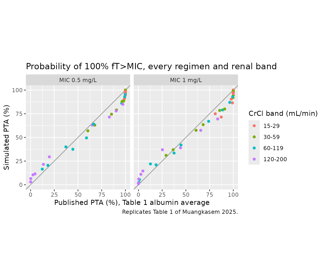
# Cells whose published PTA lies between 20% and 80% sit on the steep part of
# the attainment curve, where PTA tracks the centre of the exposure
# distribution: a wrong clearance, volume, binding constant or dose would move
# them by tens of percentage points.
mid <- cmp_t1 |> dplyr::filter(pta_paper > 20, pta_paper < 80)
cat(sprintf("mid-range cells: n = %d, median |diff| = %.1f points, median diff = %.1f points\n",
            nrow(mid), median(abs(mid$diff)), median(mid$diff)))
#> mid-range cells: n = 17, median |diff| = 4.0 points, median diff = -3.4 points
cat(sprintf("all cells: median |diff| = %.1f points, 90th pct |diff| = %.1f points\n",
            median(abs(cmp_t1$diff)), quantile(abs(cmp_t1$diff), 0.9)))
#> all cells: median |diff| = 4.7 points, 90th pct |diff| = 11.0 points
# The packaged model sits a few points below the paper in the mid-range
# (see the narrative below); the bounds leave room for that offset plus the
# 200-per-arm Monte Carlo error, while a structural error moves cells by
# tens of points.
stopifnot(
  abs(median(mid$diff)) < 10,
  median(abs(mid$diff)) < 12,
  median(abs(cmp_t1$diff)) < 10
)
Near the middle of the attainment curve, the simulated PTA agrees with Table 1 to within a few percentage points. Away from it, the published PTA is consistently more extreme than the packaged model gives. PTA is higher where attainment is likely (1 g q24h over 0.5 h at MIC 1 mg/L, 15-29 mL/min: 97.9% published vs 90.5% simulated). It is lower where attainment is unlikely (the same regimen at MIC 0.5 mg/L, 120-200 mL/min: 2.5% published vs 10.5% simulated). In other words, the paper’s simulated exposure distribution within each renal band is narrower than the published 31.4% / 23.7% / 50.6% CV interindividual variability implies. The Assumptions section below discusses this.
Neurotoxicity threshold (Table 2)
Table 2 reports the probability that the total concentration 24 h after a dose reaches 11.77 mg/L, the level associated with a 25% probability of neurological adverse effects in the cited cohort.
paper_t2 <- data.frame(
  arm_label = rep(regimens$arm_label, each = 4),
  band = factor(rep(levels(bands$band), nrow(regimens)), levels = levels(bands$band)),
  pta_paper = c(
    0.135, 0, 0, 0, 0.37, 0, 0, 0,
    91.93, 39.58, 0.02, 0, 98.515, 48.22, 0.34, 0,
    40.46, 0.525, 0, 0, 46.27, 1.31, 0, 0,
    99.99, 86.455, 35.555, 0.18, 100, 96.36, 47.46, 1.525,
    79.735, 27.505, 0.295, 0, 86.795, 35.085, 0.66, 0
  )
)
cmp_t2 <- sim |>
  dplyr::group_by(arm_label, band) |>
  dplyr::summarise(pta_sim = 100 * mean(Cc >= 11.77), .groups = "drop") |>
  dplyr::right_join(paper_t2, by = c("arm_label", "band")) |>
  dplyr::mutate(diff = pta_sim - pta_paper)
stopifnot(!anyNA(cmp_t2$pta_sim))

pick2 <- function(arm, b, col) {
  sprintf("%.1f", cmp_t2[[col]][cmp_t2$arm_label == arm & cmp_t2$band == b])
}

knitr::kable(
  cmp_t2 |>
    dplyr::select(arm_label, band, pta_paper, pta_sim) |>
    tidyr::pivot_wider(names_from = band, values_from = c(pta_paper, pta_sim)) |>
    dplyr::rename(
      "Regimen (infusion)" = arm_label,
      "15-29 paper" = `pta_paper_15-29`, "15-29 sim" = `pta_sim_15-29`,
      "30-59 paper" = `pta_paper_30-59`, "30-59 sim" = `pta_sim_30-59`,
      "60-119 paper" = `pta_paper_60-119`, "60-119 sim" = `pta_sim_60-119`,
      "120-200 paper" = `pta_paper_120-200`, "120-200 sim" = `pta_sim_120-200`
    ),
  digits = 1,
  caption = "Probability (%) of total concentration >= 11.77 mg/L at the end of the interval: Table 2 vs simulated."
)| Regimen (infusion) | 15-29 paper | 30-59 paper | 60-119 paper | 120-200 paper | 15-29 sim | 30-59 sim | 60-119 sim | 120-200 sim |
|---|---|---|---|---|---|---|---|---|
| 0.5 g q12h (0.5 h) | 91.9 | 39.6 | 0.0 | 0.0 | 74.5 | 38.0 | 8.5 | 0.0 |
| 0.5 g q12h (3 h) | 98.5 | 48.2 | 0.3 | 0.0 | 81.5 | 42.5 | 12.5 | 1.0 |
| 0.5 g q24h (0.5 h) | 0.1 | 0.0 | 0.0 | 0.0 | 11.5 | 1.5 | 0.0 | 0.0 |
| 0.5 g q24h (3 h) | 0.4 | 0.0 | 0.0 | 0.0 | 7.0 | 2.0 | 0.0 | 0.0 |
| 1 g q12h (0.5 h) | 100.0 | 86.5 | 35.6 | 0.2 | 97.0 | 77.0 | 37.5 | 6.5 |
| 1 g q12h (3 h) | 100.0 | 96.4 | 47.5 | 1.5 | 96.5 | 85.0 | 45.0 | 17.0 |
| 1 g q24h (0.5 h) | 40.5 | 0.5 | 0.0 | 0.0 | 36.5 | 11.5 | 0.5 | 0.0 |
| 1 g q24h (3 h) | 46.3 | 1.3 | 0.0 | 0.0 | 40.5 | 10.0 | 1.5 | 0.0 |
| 2 g q24h (0.5 h) | 79.7 | 27.5 | 0.3 | 0.0 | 71.5 | 29.0 | 2.5 | 0.0 |
| 2 g q24h (3 h) | 86.8 | 35.1 | 0.7 | 0.0 | 75.5 | 30.5 | 7.5 | 0.0 |
mid2 <- cmp_t2 |> dplyr::filter(pta_paper > 20, pta_paper < 80)
cat(sprintf("mid-range cells: n = %d, median diff = %.1f points, median |diff| = %.1f points\n",
            nrow(mid2), median(mid2$diff), median(abs(mid2$diff))))
#> mid-range cells: n = 9, median diff = -4.0 points, median |diff| = 4.0 points
cat(sprintf("all cells: median |diff| = %.1f points\n", median(abs(cmp_t2$diff))))
#> all cells: median |diff| = 3.2 points
stopifnot(
  abs(median(mid2$diff)) < 12,
  median(abs(cmp_t2$diff)) < 10
)
The neurotoxicity probabilities show the same pattern. The cells near 40% (1 g q24h at 15-29 mL/min, 0.5 g q12h at 30-59 mL/min, 1 g q12h at 60-119 mL/min) agree closely. The tails are again wider in the packaged model: for example, 1 g q24h over 0.5 h at 30-59 mL/min gives 11.5% simulated vs 0.5% published. For the regimens the paper recommends (Table 3), the simulated probabilities in their target bands are 11.5% (0.5 g q24h, 15-29), 11.5% (1 g q24h, 30-59), 8.5% (0.5 g q12h, 60-119) and 6.5% (1 g q12h, 120-200), against 0.02-0.53% in Table 2 and the “< 2%” stated in the abstract. The absolute neurotoxicity risk of the recommended regimens is therefore higher under the variability as published than the paper reports.
PKNCA validation
Non-compartmental analysis of 1 g every 24 h infused over 0.5 h at steady state, on total and unbound concentrations, in two arms of 200 patients at serum albumin 20 and 40 g/L with creatinine clearance uniform on 15-200 mL/min. This is the paper’s unbound-fraction calculation done per patient. At steady state the total AUC over the interval must equal Dose / CL for every patient, which checks mass balance and infusion handling. The paper reports no NCA of its own; the unbound fraction is compared against its ranges.
set.seed(20250701)
n_nca <- 200
nca_cohort <- data.frame(
  id = seq_len(2 * n_nca),
  treatment = rep(c("ALB 20 g/L", "ALB 40 g/L"), each = n_nca),
  ALB = rep(c(20, 40), each = n_nca),
  CRCL = runif(2 * n_nca, 15, 200)
)
nca_t <- sort(unique(c(seq(0, 1, by = 0.05), seq(1.25, 24, by = 0.25))))
ev_nca <- dplyr::bind_rows(
  nca_cohort |> dplyr::mutate(time = 0, amt = 1000, rate = 2000, ii = 24, ss = 1, evid = 1),
  tidyr::crossing(nca_cohort, time = nca_t) |>
    dplyr::mutate(amt = 0, rate = 0, ii = 0, ss = 0, evid = 0)
) |>
  dplyr::mutate(cmt = "central") |>
  dplyr::arrange(id, time, dplyr::desc(evid))

rxode2::rxSetSeed(20250701)
sim_nca <- rxode2::rxSolve(ui, ev_nca, returnType = "data.frame",
                           keep = "treatment", maxsteps = 1e6)
stopifnot(!anyNA(sim_nca$Cc))
dose_df <- ev_nca |>
  dplyr::filter(evid == 1) |>
  dplyr::select(id, time, amt, treatment)
intervals <- data.frame(start = 0, end = 24, cmax = TRUE, tmax = TRUE,
                        cmin = TRUE, auclast = TRUE, cav = TRUE)

run_nca <- function(conc_col) {
  # A subject that fails to solve comes back NA; stop rather than drop it.
  stopifnot(!anyNA(sim_nca[[conc_col]]))
  conc <- sim_nca |>
    dplyr::filter(!is.na(.data[[conc_col]])) |>
    dplyr::transmute(id, time, treatment, conc = .data[[conc_col]])
  o_conc <- PKNCA::PKNCAconc(conc, conc ~ time | treatment + id)
  o_dose <- PKNCA::PKNCAdose(dose_df, amt ~ time | treatment + id)
  as.data.frame(PKNCA::pk.nca(PKNCA::PKNCAdata(o_conc, o_dose, intervals = intervals))$result)
}
nca_tot <- run_nca("Cc")
nca_unb <- run_nca("Cunbound")

nca_summary <- dplyr::bind_rows(
  nca_tot |> dplyr::mutate(analyte = "total"),
  nca_unb |> dplyr::mutate(analyte = "unbound")
) |>
  dplyr::group_by(analyte, treatment, PPTESTCD) |>
  dplyr::summarise(median = median(PPORRES), .groups = "drop") |>
  tidyr::pivot_wider(names_from = PPTESTCD, values_from = median)

knitr::kable(
  nca_summary |>
    dplyr::select(analyte, treatment, cmax, tmax, cmin, auclast, cav) |>
    dplyr::rename("Analyte" = analyte, "Group" = treatment,
                  "Cmax (mg/L)" = cmax, "Tmax (h)" = tmax,
                  "Cmin (mg/L)" = cmin, "AUC0-24 (mg*h/L)" = auclast,
                  "Cavg (mg/L)" = cav),
  digits = 2,
  caption = "Median steady-state NCA parameters, 1 g q24h over 0.5 h (simulated)."
)| Analyte | Group | Cmax (mg/L) | Tmax (h) | Cmin (mg/L) | AUC0-24 (mg*h/L) | Cavg (mg/L) |
|---|---|---|---|---|---|---|
| total | ALB 20 g/L | 75.07 | 0.5 | 0.79 | 329.10 | 13.71 |
| total | ALB 40 g/L | 74.16 | 0.5 | 0.76 | 327.00 | 13.63 |
| unbound | ALB 20 g/L | 46.25 | 0.5 | 0.24 | 145.56 | 6.07 |
| unbound | ALB 40 g/L | 37.86 | 0.5 | 0.32 | 150.19 | 6.26 |
auc_chk <- nca_tot |>
  dplyr::filter(PPTESTCD == "auclast") |>
  dplyr::left_join(sim_nca |> dplyr::distinct(id, cl), by = "id") |>
  dplyr::mutate(rel_err = PPORRES * cl / 1000 - 1)
cat(sprintf("AUC0-24 x CL / Dose - 1: median %.2g, 90th pct |err| %.2g\n",
            median(auc_chk$rel_err), quantile(abs(auc_chk$rel_err), 0.9)))
#> AUC0-24 x CL / Dose - 1: median 6.1e-05, 90th pct |err| 0.00018
# Trapezoidal error on this grid is well under 1%; a wrong clearance, dose or
# infusion handling moves the ratio by tens of percent.
stopifnot(abs(median(auc_chk$rel_err)) < 0.01,
          quantile(abs(auc_chk$rel_err), 0.9) < 0.02)
fu_ind <- nca_unb |>
  dplyr::filter(PPTESTCD == "auclast") |>
  dplyr::select(id, treatment, auc_u = PPORRES) |>
  dplyr::left_join(nca_tot |> dplyr::filter(PPTESTCD == "auclast") |>
                     dplyr::select(id, auc_t = PPORRES), by = "id") |>
  dplyr::left_join(nca_cohort |> dplyr::select(id, CRCL), by = "id") |>
  dplyr::mutate(fu = auc_u / auc_t)

fu_tab <- fu_ind |>
  dplyr::group_by(treatment) |>
  dplyr::summarise(median = median(fu), p05 = quantile(fu, 0.05),
                   p95 = quantile(fu, 0.95), .groups = "drop") |>
  dplyr::mutate(published = c("0.37-0.56", "0.44-0.49"))

knitr::kable(
  fu_tab |>
    dplyr::rename("Group" = treatment, "Median fu" = median,
                  "5th pct" = p05, "95th pct" = p95,
                  "Published range" = published),
  digits = 3,
  caption = "Per-patient unbound fraction (AUCu / AUC, PKNCA) vs the Results ranges."
)| Group | Median fu | 5th pct | 95th pct | Published range |
|---|---|---|---|---|
| ALB 20 g/L | 0.450 | 0.406 | 0.511 | 0.37-0.56 |
| ALB 40 g/L | 0.462 | 0.450 | 0.482 | 0.44-0.49 |
# The median sits well inside each published range; the tails depend on
# which patients draw extreme clearances and are not asserted.
stopifnot(
  fu_tab$median[1] > 0.37, fu_tab$median[1] < 0.56,
  fu_tab$median[2] > 0.44, fu_tab$median[2] < 0.49
)

ggplot(fu_ind, aes(CRCL, fu, colour = treatment)) +
  geom_point(alpha = 0.5) +
  geom_hline(yintercept = c(0.37, 0.56), linetype = "dashed", colour = "#E69F00") +
  geom_hline(yintercept = c(0.44, 0.49), linetype = "dotted", colour = "#56B4E9") +
  scale_colour_manual(values = c("ALB 20 g/L" = "#E69F00", "ALB 40 g/L" = "#56B4E9")) +
  labs(x = "Cockcroft-Gault creatinine clearance (mL/min)",
       y = "Unbound fraction (AUCu / AUC)", colour = NULL,
       title = "Steady-state unbound fraction, 1 g q24h over 0.5 h",
       caption = "Lines: published ranges at 20 g/L (dashed) and 40 g/L (dotted).")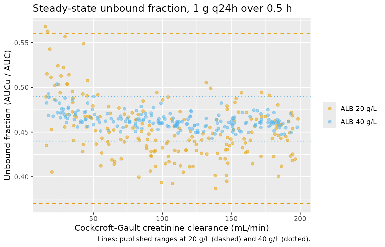
Assumptions and deviations
- Composite model. The structural PK parameters and their variability are the Burkhardt 2007 values as printed in this paper; they were not re-estimated and are encoded as fixed. Only the creatinine clearance exponent (0.535) and the four albumin-binding coefficients were estimated by the authors, each by least-squares regression on digitised data from a different study. Their precision is reported only as r^2 (0.81, 0.99 and 1).
-
Residual error. The paper performs simulation only
and reports no residual error model.
propSdis fixed to zero rather than invented, so simulated concentrations are individual predictions, which is also what PTA analyses use. -
IIV form. The paper gives interindividual
variability as percentages. They are read as coefficients of variation
of log-normal random effects,
omega^2 = log(1 + CV^2). Reading them as standard deviations on the log scale instead (omega^2 = CV^2) changes the variances by less than 5%. That is far too small to explain the narrower tails of the published PTA tables. No eta is placed on Q (published IIV 0%). - Narrower published tails. Halving the variances, or even cutting them to a quarter, narrows the gap with Tables 1 and 2 but does not close it. The paper does not report the sampling distribution of creatinine clearance within its bands, how Simulx was parameterised, or a seed, and its own Figure S2 VPC shows the variability it used only graphically. The packaged model therefore carries the variability as printed, and is not tuned to the tables. The central tendency, which drives the authors’ dose recommendations, is reproduced.
- Covariate distributions. Creatinine clearance is drawn uniformly within each renal band and albumin uniformly on 20-40 g/L (the uniform albumin draw is supported by the Bmax and KD quartiles; the creatinine clearance draw is an assumption). Each regimen-by-band arm has 200 patients instead of a single 10,000-patient population.
- Steady state. Both targets are read at steady state at the end of the dosing interval. The paper does not say whether its PTA used the first dose or steady state. A first-dose reading gives similar efficacy PTA and lower neurotoxicity probabilities; the steady-state reading reproduces the near-40% neurotoxicity cells of Table 2 more closely.
- Equation 1 reference. The paper does not say what statistic the 78 mL/min normalising constant is; it is used exactly as printed.
- Albumin extrapolation. The binding model was fitted to patients with albumin 24-30 g/L. Like the paper, this vignette extrapolates it to 20-40 g/L.
- Albumin-band resolution. Table 1 is compared after averaging over its four albumin sub-bands, because 200 patients per arm cannot resolve the 1-5 percentage-point albumin effects.