Abacavir (Jullien 2005)
Source:vignettes/articles/Jullien_2005_abacavir.Rmd
Jullien_2005_abacavir.RmdModel and source
- Citation: Jullien V, Treluyer J-M, Chappuy H, Dimet J, Rey E, Dupin N, Salmon D, Pons G, Urien S. Weight related differences in the pharmacokinetics of abacavir in HIV-infected patients. Br J Clin Pharmacol. 2005;59(2):183-188. doi:10.1111/j.1365-2125.2004.02259.x
- Description: Two-compartment population PK model for abacavir in HIV-infected adults (Jullien 2005); apparent clearance scales with body weight via an estimated power exponent, Q/F is fixed when BW is added to the model
- Article: https://doi.org/10.1111/j.1365-2125.2004.02259.x
Population
Jullien et al. (2005) developed a population PK model for oral abacavir from routine therapeutic-drug-monitoring data in 188 HIV-infected adults (151 men, 37 women) at a single Paris hospital. All subjects received the recommended 300 mg BID abacavir tablet dose as part of highly active antiretroviral therapy. Age ranged 16.1-72.8 years (median 40), body weight ranged 36-102 kg (median 65), and 344 plasma samples were collected with a median of one sample per patient (range 1-7, mean 1.9). Thirty samples were below the analytical limit of quantification (LOQ 0.01 mg/L) and were imputed at half the LOQ. See Jullien 2005 Table 1 for the full baseline demographic summary.
The same information is available programmatically via the model’s
population metadata
(readModelDb("Jullien_2005_abacavir")$population).
Source trace
The per-parameter origin is recorded as an in-file comment next to
each ini() entry in
inst/modeldb/specificDrugs/Jullien_2005_abacavir.R. The
table below collects them in one place for review.
| Equation / parameter | Value | Source location |
|---|---|---|
lka (Ka) |
log(1.8) (1/h) | Table 3, TV(Ka) = 1.8 1/h |
lcl (CL/F at 65 kg) |
log(47.5) (L/h) | Table 3, TV(CL/F) = 47.5 L/h |
lvc (Vc/F) |
log(75) (L) | Table 3, TV(Vc/F) = 75 L |
lvp (Vp/F) |
log(24) (L) | Table 3, TV(Vp/F) = 24 L |
lq (Q/F, fixed) |
log(10) (L/h) | Table 3, TV(Q/F) = 10 L/h (fixed at basic-model typical value when BW added to CL/F) |
e_wt_cl |
0.80 | Table 3, theta_BW = 0.80 |
| IIV CL/F (omega^2) | 0.18 | Table 3, omega^2_CL/F = 0.18 |
| IIV Vc/F (omega^2) | 0.51 | Table 3, omega^2_Vc/F = 0.51 |
| IIV Ka (omega^2) | 1.13 | Table 3, omega^2_Ka = 1.13 |
| Cov(CL/F, Vc/F) | 0.27 | Table 3, COV(CL,V) = 0.27 |
addSd (residual SD) |
sqrt(0.039) ~= 0.1975 (mg/L) | Table 3, sigma^2 = 0.039 (mg/L)^2 |
d/dt(depot) |
-ka * depot | Methods, two-compartment first-order absorption |
d/dt(central) |
ka * depot - kel * central - k12 * central + k21 * peripheral1 | Methods (ADVAN4 TRANS4) |
d/dt(peripheral1) |
k12 * central - k21 * peripheral1 | Methods |
| Covariate model on CL/F | CL/F = TV(CL/F) * (WT/65)^theta_BW | Methods, covariate submodel (median BW = 65 kg) |
Virtual cohort
Original observed data from the routine therapeutic-drug-monitoring study are not publicly available. The simulations below use a virtual cohort of 188 adults whose body-weight distribution approximates Jullien 2005 Table 1 (mean 65.4 kg, SD 12.3 kg, range 36-102 kg). Body weight is sampled from a truncated normal matching those moments; female fraction is set to 19.7%.
set.seed(20250604)
n_subj <- 188L

draw_wt <- function(n, mean_wt = 65.4, sd_wt = 12.3, lo = 36, hi = 102) {
  wt <- numeric(0)
  while (length(wt) < n) {
    cand <- rnorm(n * 2L, mean_wt, sd_wt)
    cand <- cand[cand >= lo & cand <= hi]
    wt <- c(wt, cand)
  }
  wt[seq_len(n)]
}

cohort <- tibble(
  id   = seq_len(n_subj),
  WT   = round(draw_wt(n_subj), 1),
  SEXF = rbinom(n_subj, 1, prob = 37 / 188)
)

# Stratify into the BW bands used in Jullien 2005 Figure 3A so per-band
# AUC can be compared against the published means.
cohort <- cohort |>
  mutate(
    wt_band = cut(
      WT,
      breaks = c(-Inf, 50, 60, 70, 80, Inf),
      labels = c("<50", "50-60", "60-70", "70-80", ">80"),
      right  = FALSE
    )
  )

knitr::kable(
  cohort |> count(wt_band, name = "n_subjects"),
  caption = "Virtual cohort distribution across the Jullien 2005 Figure 3A bodyweight bands."
)| wt_band | n_subjects |
|---|---|
| <50 | 18 |
| 50-60 | 58 |
| 60-70 | 57 |
| 70-80 | 35 |
| >80 | 20 |
Simulation
Steady-state abacavir 300 mg BID for seven days (14 doses, q12h), with observations every 0.25 h over the final 12 h dosing interval.
mod <- rxode2::rxode2(readModelDb("Jullien_2005_abacavir"))
#> ℹ parameter labels from comments will be replaced by 'label()'

tau     <- 12              # dosing interval (h)
ndose   <- 14L             # 7 days BID = 14 doses
dose_mg <- 300

dose_times <- seq(from = 0, by = tau, length.out = ndose)
ss_start   <- (ndose - 1L) * tau   # time of the final dose
obs_times  <- seq(ss_start, ss_start + tau, by = 0.25)

build_events <- function(cohort_df) {
  dose_rows <- cohort_df |>
    tidyr::expand_grid(time = dose_times) |>
    mutate(evid = 1L, amt = dose_mg, cmt = "depot", Cc = NA_real_)

  obs_rows <- cohort_df |>
    tidyr::expand_grid(time = obs_times) |>
    mutate(evid = 0L, amt = 0, cmt = NA_character_, Cc = NA_real_)

  bind_rows(dose_rows, obs_rows) |>
    arrange(id, time, evid)
}

events <- build_events(cohort)

sim <- rxode2::rxSolve(mod, events = events,
                       keep = c("WT", "SEXF", "wt_band")) |>
  as.data.frame() |>
  filter(time >= ss_start) |>
  mutate(time_after_dose = time - ss_start)
A deterministic typical-value replication uses
rxode2::zeroRe() so figures that show the
population-typical curve do not carry between-subject spread.
mod_typical <- mod |> rxode2::zeroRe()

typical_cohort <- tibble(
  id      = seq_len(5L),
  WT      = c(40, 55, 65, 80, 95),
  SEXF    = 0L,
  wt_band = factor(c("<50", "50-60", "60-70", "70-80", ">80"),
                   levels = c("<50", "50-60", "60-70", "70-80", ">80"))
)

events_typical <- build_events(typical_cohort)

sim_typical <- rxode2::rxSolve(mod_typical, events = events_typical,
                               keep = c("WT", "wt_band")) |>
  as.data.frame() |>
  filter(time >= ss_start) |>
  mutate(time_after_dose = time - ss_start)
#> ℹ omega/sigma items treated as zero: 'etalcl', 'etalvc', 'etalka'
#> Warning: multi-subject simulation without without 'omega'
Replicate published figures
Figure 1 – concentration vs. time after dose
Figure 1 of Jullien 2005 shows individual observed abacavir concentrations versus time after dose, overlaid with the typical population PK curve. The virtual-cohort simulation reproduces the shape of the typical curve and the spread of individual trajectories over a single 12 h dosing interval at steady state.
typical_curve <- sim_typical |> filter(WT == 65)

ggplot() +
  geom_line(
    data    = sim |> filter(id <= 30L),
    mapping = aes(time_after_dose, Cc, group = id),
    alpha   = 0.25
  ) +
  geom_line(
    data    = typical_curve,
    mapping = aes(time_after_dose, Cc),
    colour  = "firebrick",
    linewidth = 1
  ) +
  labs(
    x = "Time after dose (h)",
    y = "Abacavir concentration (mg/L)",
    title = "Figure 1 -- abacavir concentration vs. time after dose",
    subtitle = "Thin lines: 30 simulated subjects; thick line: typical 65 kg subject",
    caption = "Replicates Figure 1 of Jullien 2005."
  )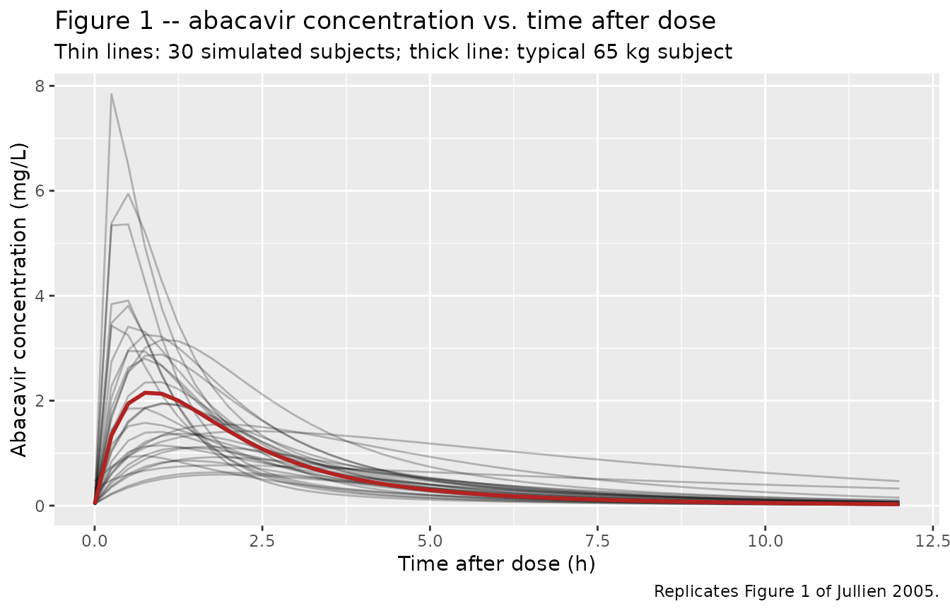
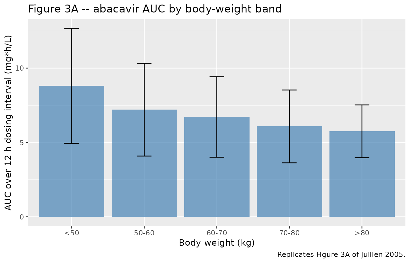
Figure 3A – AUC vs. body-weight band
Figure 3A of Jullien 2005 shows the mean +/- SD steady-state abacavir AUC across five body-weight bands. AUC declines monotonically with body weight because apparent clearance scales as (WT/65)^0.80.
trapz <- function(t, y) {
  ord <- order(t)
  t <- t[ord]; y <- y[ord]
  sum(diff(t) * (head(y, -1) + tail(y, -1)) / 2)
}

auc_by_subject <- sim |>
  group_by(id, wt_band, WT) |>
  summarise(
    AUC = trapz(time_after_dose, Cc),
    .groups = "drop"
  )

auc_summary <- auc_by_subject |>
  group_by(wt_band) |>
  summarise(
    n      = dplyr::n(),
    mean   = mean(AUC),
    sd     = sd(AUC),
    .groups = "drop"
  )

ggplot(auc_summary, aes(wt_band, mean)) +
  geom_col(fill = "steelblue", alpha = 0.7) +
  geom_errorbar(aes(ymin = pmax(mean - sd, 0), ymax = mean + sd), width = 0.2) +
  labs(
    x = "Body weight (kg)",
    y = "AUC over 12 h dosing interval (mg*h/L)",
    title = "Figure 3A -- abacavir AUC by body-weight band",
    caption = "Replicates Figure 3A of Jullien 2005."
  )
knitr::kable(
  auc_summary,
  digits = c(0, 0, 2, 2),
  caption = "Simulated steady-state abacavir AUC (mean +/- SD) by Jullien 2005 body-weight band."
)| wt_band | n | mean | sd |
|---|---|---|---|
| <50 | 18 | 8.81 | 3.87 |
| 50-60 | 58 | 7.20 | 3.12 |
| 60-70 | 57 | 6.72 | 2.71 |
| 70-80 | 35 | 6.08 | 2.45 |
| >80 | 20 | 5.75 | 1.77 |
PKNCA validation
The simulated steady-state concentrations are summarised with PKNCA so the per-band AUC, Cmax, Tmax, and Cmin values are computed by a standard NCA engine rather than ad hoc.
sim_nca <- sim |>
  filter(!is.na(Cc)) |>
  select(id, time, Cc, wt_band) |>
  mutate(wt_band = as.character(wt_band))

dose_df <- events |>
  filter(evid == 1L, time == ss_start) |>
  select(id, time, amt) |>
  inner_join(cohort |> select(id, wt_band) |>
               mutate(wt_band = as.character(wt_band)),
             by = "id")

conc_obj <- PKNCA::PKNCAconc(sim_nca, Cc ~ time | wt_band + id,
                             concu = "mg/L", timeu = "h")
dose_obj <- PKNCA::PKNCAdose(dose_df, amt ~ time | wt_band + id,
                             doseu = "mg")

intervals <- data.frame(
  start    = ss_start,
  end      = ss_start + tau,
  cmax     = TRUE,
  tmax     = TRUE,
  cmin     = TRUE,
  auclast  = TRUE,
  cav      = TRUE
)

nca_res <- PKNCA::pk.nca(PKNCA::PKNCAdata(conc_obj, dose_obj,
                                          intervals = intervals))

nca_tbl <- as.data.frame(nca_res$result) |>
  filter(PPTESTCD %in% c("cmax", "tmax", "cmin", "auclast", "cav")) |>
  group_by(wt_band, PPTESTCD) |>
  summarise(median = median(PPORRES, na.rm = TRUE),
            .groups = "drop") |>
  tidyr::pivot_wider(names_from = PPTESTCD, values_from = median)

knitr::kable(
  nca_tbl,
  digits = 3,
  caption = "PKNCA-derived steady-state NCA per Jullien 2005 body-weight band (one 12 h dosing interval at day 7)."
)| wt_band | auclast | cav | cmax | cmin | tmax |
|---|---|---|---|---|---|
| 50-60 | 6.502 | 0.542 | 1.970 | 0.047 | 0.75 |
| 60-70 | 6.061 | 0.505 | 1.741 | 0.037 | 0.75 |
| 70-80 | 5.734 | 0.478 | 1.952 | 0.032 | 1.00 |
| <50 | 8.099 | 0.675 | 2.432 | 0.066 | 0.75 |
| >80 | 5.834 | 0.486 | 1.898 | 0.022 | 0.75 |
Comparison against published NCA
Jullien 2005 reports mean +/- SD AUC declining from 10.7 +/- 5.0 mgh/L in the lightest subjects (around 36 kg) to 5.7 +/- 1.6 mgh/L in the heaviest (around 102 kg). They also cite a population target AUC of about 6 mg*h/L for adequate antiviral exposure. The simulated AUC means above should reproduce the same monotonically decreasing trend across the five bands and fall within the ranges anchoring the lightest and heaviest groups.
published <- tibble::tibble(
  wt_band = c("<50", "50-60", "60-70", "70-80", ">80"),
  AUC_pub_mean_text = c(
    "approx 10.7 (lightest band; SD 5.0)",
    "intermediate",
    "intermediate",
    "intermediate",
    "approx 5.7 (heaviest band; SD 1.6)"
  )
)

comparison <- auc_summary |>
  mutate(wt_band = as.character(wt_band)) |>
  left_join(published, by = "wt_band") |>
  select(wt_band, n, sim_AUC_mean = mean, sim_AUC_sd = sd,
         published_AUC = AUC_pub_mean_text)

knitr::kable(
  comparison,
  digits = c(0, 0, 2, 2, 0),
  caption = "Simulated vs. published per-band AUC. Jullien 2005 anchors only the lightest and heaviest bands as numeric means; intermediate bands are reported graphically in Figure 3A."
)| wt_band | n | sim_AUC_mean | sim_AUC_sd | published_AUC |
|---|---|---|---|---|
| <50 | 18 | 8.81 | 3.87 | approx 10.7 (lightest band; SD 5.0) |
| 50-60 | 58 | 7.20 | 3.12 | intermediate |
| 60-70 | 57 | 6.72 | 2.71 | intermediate |
| 70-80 | 35 | 6.08 | 2.45 | intermediate |
| >80 | 20 | 5.75 | 1.77 | approx 5.7 (heaviest band; SD 1.6) |
Assumptions and deviations
- The published cohort had 1.9 plasma samples per patient on average (range 1-7) from routine TDM, while the simulation samples densely at steady state (every 0.25 h over a 12 h dosing interval). The richer simulated sampling is appropriate for verifying the structural model but does not reproduce the sparse-sampling design of the original study.
- The original data carried 30 BLQ observations imputed at half the LOQ (0.005 mg/L). The simulation has no BLQ handling because the deterministic ODE simulation produces continuous positive concentrations.
- Body-weight distribution is sampled from a truncated normal whose mean and SD match Table 1 (65.4 kg, 12.3 kg) and whose support is constrained to the published range (36-102 kg). Age and concomitant antiretroviral therapy are not modelled because the source paper tested but did not retain age, gender, dose-per-unit-bodyweight, NRTI co-medication, NNRTI co-medication, or PI co-medication as covariates on any structural parameter (Results, p.185).
- Interindividual variability on Q/F and Vp/F could not be estimated
in the source publication and is therefore omitted from the model (no
etalqoretalvp). Q/F itself was fixed at the basic-model typical value of 10 L/h when body weight was added to CL/F. - The published residual variability is reported as sigma^2 = 0.039
(mg/L)^2 on the additive (linear-concentration) scale; the model encodes
addSd = sqrt(0.039) ~= 0.1975 mg/Laccordingly. No log-additive or proportional residual component is included. - The bootstrap-validation column of Jullien 2005 Table 3 is reported only in the source for diagnostic purposes; the model uses the original-dataset point estimates as the canonical values.