Metronidazole (Randell 2024)
Source:vignettes/articles/Randell_2024_metronidazole.Rmd
Randell_2024_metronidazole.RmdModel and source
- Citation: Randell RL, Balevic SJ, Greenberg RG, Cohen-Wolkowiez M, Thompson EJ, Venkatachalam S, Smith MJ, Bendel C, Bliss JM, Chaaban H, Chhabra R, Dammann CEL, Downey LC, Hornik C, Hussain N, Laughon MM, Lavery A, Moya F, Saxonhouse M, Sokol GM, Trembath A, Weitkamp J-H, Hornik CP. Opportunistic dried blood spot sampling validates and optimizes a pediatric population pharmacokinetic model of metronidazole. Antimicrob Agents Chemother. 2024;68(4):e01533-23. doi:10.1128/aac.01533-23. Erratum: Antimicrob Agents Chemother. 2025;69(9):e00972-25. doi:10.1128/aac.00972-25 (Table 1 Hill parameter: ‘7’ should read ‘15.7’).
- Description: One-compartment intravenous population PK model for metronidazole in critically ill preterm and term infants (Randell 2024, ‘optimized model’). Clearance scales linearly with body weight and matures with postmenstrual age through a sigmoidal Emax (Hill) function (TM50 25.6 weeks, Hill 15.7); central volume scales with body weight through an estimated power exponent (0.763). The model was developed by externally validating and then optimizing the PTN_METRO model of Cohen-Wolkowiez 2013 using estimated plasma concentrations derived from opportunistically collected dried blood spots.
- Article: https://doi.org/10.1128/aac.01533-23
- Erratum: https://doi.org/10.1128/aac.00972-25
- Supplement (Tables S1-S3, Figures S1-S5):
AAC01533-23-s0001.docx, linked from the article’s “Additional Files” section.
The erratum is load-bearing for this model. Table 1 of the 2024
article prints the Hill coefficient of the clearance maturation function
as 7; the 2025 erratum corrects it to 15.7.
The printed value of 7 is outside the paper’s own bootstrap interval for
that parameter (2.5th-97.5th percentile 8.4-41.0, median 15.9), which
independently corroborates the correction. This model file uses
15.7.
Population
The optimized model was fit to a combined data set assembled from two Pediatric Trials Network studies (Randell 2024 Table S1):
- PTN_METRO (Metronidazole Pharmacokinetics in Premature Infants, NCT01222585) contributed measured plasma metronidazole concentrations. 24 infants appear in the combined demographics table; 42 paired dried-blood-spot (DBS) and plasma samples from 21 of these infants were used for the comparability analysis.
-
SCAMP (Antibiotic Safety in Infants with
Complicated Intra-Abdominal Infections, NCT01994993) contributed 122
infants and 399 DBS. DBS concentrations were converted to estimated
plasma concentrations (ePlasma) with the comparability regression
Cplasma = 1.11 * CDBS + 253ng/mL (R-squared 0.86).
Combined cohort (n = 146), reported as mean (SD):
- Gestational age at birth: 30.6 (5.2) weeks; supported range 22.7-41.0 weeks.
- Postnatal age: 18.6 (17.3) days; supported range 0-80 days.
- Postmenstrual age: 33.2 (5.3) weeks; supported range 23-48 weeks.
- Weight: 1.8 (1.0) kg.
- Serum creatinine: 0.6 (0.4) mg/dL.
- Albumin: 2.4 (0.6) g/dL (n = 101).
- Sex: 81 of 146 (55 percent) male, i.e., 45 percent female.
- Race / ethnicity: 88 of 146 (60 percent) White; 30 of 146 (21 percent) Hispanic ethnicity.
In the SCAMP trial metronidazole was given as a 30-minute intravenous infusion: a 15 mg/kg loading dose, a 7.5 mg/kg maintenance dose at 24 hours, and subsequent 7.5 mg/kg maintenance doses at postmenstrual-age-defined intervals (every 12 h for PMA 23 to less than 34 weeks, every 8 h for PMA 34-40 weeks, every 6 h for PMA greater than 40 weeks).
The same information is available programmatically via the model’s
population metadata
(readModelDb("Randell_2024_metronidazole")()$population).
Source trace
The per-parameter origin is recorded as an in-file comment next to
each ini() entry in
inst/modeldb/specificDrugs/Randell_2024_metronidazole.R.
The table below collects them in one place for review.
| Equation / parameter | Value | Source location |
|---|---|---|
| Structural model: 1-compartment IV (NONMEM ADVAN1 TRANS2) | n/a | Methods, “Optimization”; Table 1 structural-model rows |
CL = theta_CL * WT * [PMA^Hill / (TM50^Hill + PMA^Hill)] |
n/a | Table 1, structural-model row |
V = theta_V * WT^theta_WT-V |
n/a | Table 1, structural-model row |
lcl = log(0.036) (theta_CL, L/h/kg) |
0.036 | Table 1, “theta_CL (L/kg/h)”; RSE 4 percent, bootstrap 0.033-0.039 |
lvc = log(0.853) (theta_V, L at WT = 1 kg) |
0.853 | Table 1, “theta_V (L/kg)”; RSE 3 percent, bootstrap 0.802-0.921 |
e_wt_cl = fixed(1) |
1 | Methods, “Optimization”: CLi = CL * WT^1 with a fixed
exponent; Table 1 structural row CL = theta_CL * WT
|
e_wt_vc = 0.763 (theta_WT-V) |
0.763 | Table 1, “theta_WT-V”; RSE 8 percent, bootstrap 0.645-0.876 |
pma50_cl = 25.6 (TM50, weeks) |
25.6 | Table 1, “TM50 (weeks)”; RSE 2 percent, bootstrap 24.4-26.5 |
hill_cl = 15.7 (Hill) |
15.7 | Table 1, “Hill”, as corrected by the 2025 erratum (doi:10.1128/aac.00972-25); Table 1 as printed in 2024 reads 7. RSE 37 percent, bootstrap 8.4-41.0 |
etalcl variance 0.11933 |
omega^2 = log(1 + 0.356^2) | Table 1, “Interindividual variability (%CV) CL = 35.6”; RSE 21 percent, eta shrinkage 8 percent |
etalvc variance 0.06252 |
omega^2 = log(1 + 0.254^2) | Table 1, “Interindividual variability (%CV) V = 25.4”; RSE 31 percent, eta shrinkage 29 percent |
propSd = 0.191 |
19.1 percent | Table 1, “Residual error, Proportional error (%)”; RSE 13 percent, epsilon shrinkage 17 percent |
pma_wk = PAGE * 4.35 |
n/a | Unit conversion only: the canonical PAGE covariate is
in months and the paper’s TM50 is in weeks |
d/dt(central) = -kel * central,
Cc = central / vc
|
n/a | One-compartment IV disposition (Methods, “Optimization”) |
Values reported by the paper only as diagnostics (eta and epsilon shrinkage, RSEs, bootstrap percentiles) are recorded in the comments but are not model parameters.
The correction from the erratum
The maturation function is extremely steep, so the difference between the printed Hill coefficient (7) and the corrected one (15.7) is not cosmetic: it changes the predicted fraction of mature clearance by up to roughly 20 percentage points in the age range where most of the cohort sits.
fmat <- function(pma_wk, hill, tm50 = 25.6) {
  pma_wk^hill / (tm50^hill + pma_wk^hill)
}

pma_grid <- seq(22, 48, by = 0.25)

maturation <- dplyr::bind_rows(
  tibble::tibble(pma_wk = pma_grid, fmat = fmat(pma_grid, 15.7),
                 source = "Hill = 15.7 (erratum; used here)"),
  tibble::tibble(pma_wk = pma_grid, fmat = fmat(pma_grid, 7),
                 source = "Hill = 7 (as printed in Table 1)")
)

ggplot(maturation, aes(pma_wk, fmat, colour = source)) +
  geom_line() +
  labs(x = "Postmenstrual age (weeks)",
       y = "Fraction of mature clearance",
       colour = NULL,
       caption = "Maturation term of Randell 2024 Table 1 under the printed and corrected Hill coefficients.") +
  theme(legend.position = "bottom")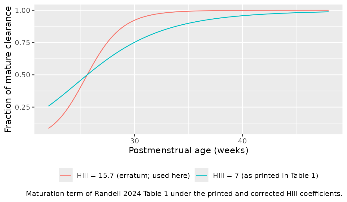
The largest absolute difference between the two curves over the supported 23-48 week PMA range is 0.173.
Virtual cohort
Original observed concentrations are not publicly available. The simulations below use virtual cohorts whose covariate distributions approximate the published trial demographics, dosed with the postmenstrual-age-based regimen the paper evaluates.
set.seed(1533)

# Build one PMA-band cohort as a self-contained event table.
#
# Dosing follows the SCAMP protocol (Randell 2024, Methods "Study design and
# sample collection"): a 15 mg/kg loading dose at time 0, a 7.5 mg/kg
# maintenance dose at 24 h, then 7.5 mg/kg every tau_h through the end of the
# dosing window. Every dose is a 30-minute infusion, encoded via `rate`.
#
# `id_offset` shifts subject IDs so cohorts stay disjoint when bound together;
# duplicate IDs would silently collapse into single (wrong) subjects.
INFUSION_H <- 0.5
DOSE_END_H <- 120  # last maintenance dose
OBS_END_H  <- 168  # observation continues 48 h past the last dose

make_cohort <- function(n, pma_week_lo, pma_week_hi, wt_kg_lo, wt_kg_hi,
                        tau_h, treatment, id_offset = 0L) {
  subj <- tibble::tibble(
    id        = id_offset + seq_len(n),
    WT        = runif(n, wt_kg_lo, wt_kg_hi),
    pma_wk    = runif(n, pma_week_lo, pma_week_hi),
    treatment = treatment
  ) |>
    dplyr::mutate(PAGE = pma_wk / 4.35)

  maint_times <- seq(24, DOSE_END_H, by = tau_h)
  obs_times   <- seq(0, OBS_END_H, by = 1)

  dose_rows <- subj |>
    tidyr::expand_grid(time = c(0, maint_times)) |>
    dplyr::mutate(
      amt  = WT * dplyr::if_else(time == 0, 15, 7.5),
      rate = amt / INFUSION_H,
      evid = 1L,
      cmt  = "central"
    )

  obs_rows <- subj |>
    tidyr::expand_grid(time = obs_times) |>
    dplyr::mutate(amt = NA_real_, rate = NA_real_, evid = 0L, cmt = "central")

  dplyr::bind_rows(dose_rows, obs_rows) |>
    dplyr::arrange(id, time, dplyr::desc(evid)) |>
    dplyr::select(id, time, amt, rate, evid, cmt, WT, PAGE, treatment) |>
    as.data.frame()
}

# The three PMA bands of the dosing guideline the paper evaluates, plus a
# counterfactual: the oldest band dosed on the youngest band's 12-hourly
# interval. Weight ranges bracket the combined-cohort mean of 1.8 kg and widen
# with PMA. The counterfactual arm reuses the >40 wk covariate distribution and
# the same seed-stream position is irrelevant because each arm draws its own
# covariates.
ARM_LEVELS <- c("PMA 23 to <34 wk (q12h)", "PMA 34-40 wk (q8h)",
                "PMA >40 wk (q6h)", "PMA >40 wk (q12h, counterfactual)")

events <- dplyr::bind_rows(
  make_cohort(n = 150, pma_week_lo = 23, pma_week_hi = 34,
              wt_kg_lo = 0.6, wt_kg_hi = 2.2, tau_h = 12,
              treatment = ARM_LEVELS[1], id_offset =   0L),
  make_cohort(n = 150, pma_week_lo = 34, pma_week_hi = 40,
              wt_kg_lo = 1.5, wt_kg_hi = 3.4, tau_h = 8,
              treatment = ARM_LEVELS[2], id_offset = 150L),
  make_cohort(n = 150, pma_week_lo = 40, pma_week_hi = 48,
              wt_kg_lo = 2.4, wt_kg_hi = 5.0, tau_h = 6,
              treatment = ARM_LEVELS[3], id_offset = 300L),
  make_cohort(n = 150, pma_week_lo = 40, pma_week_hi = 48,
              wt_kg_lo = 2.4, wt_kg_hi = 5.0, tau_h = 12,
              treatment = ARM_LEVELS[4], id_offset = 450L)
)

# Guard: IDs must be disjoint across cohorts and (id, time, evid) unique.
stopifnot(
  nrow(dplyr::distinct(events, id, time, evid)) == nrow(events),
  dplyr::n_distinct(events$id) == 600L
)
Simulation
mod <- readModelDb("Randell_2024_metronidazole")

sim <- rxode2::rxSolve(
  mod,
  events = events,
  keep   = c("treatment", "WT", "PAGE")
) |>
  as.data.frame()
#> ℹ parameter labels from comments will be replaced by 'label()'
Closed-form validation gates
Before looking at any figure, the packaged model is checked against
the closed-form results that a one-compartment linear model must satisfy
exactly. These gates use rxode2::zeroRe() so the checks run
on the typical-value profile rather than a population median (which a
log-normal eta would bias).
Gate 1 - steady-state exposure equals dose divided by clearance
For any linear one-compartment model at steady state,
AUC(tau) = Dose / CL regardless of the input mode. The gate
below reconstructs CL from the published parameters and
compares it against the AUC that PKNCA computes over a steady-state
dosing interval (ss = 1).
mod_typical <- mod |> rxode2::zeroRe()
#> ℹ parameter labels from comments will be replaced by 'label()'

# Typical subjects spanning the supported PMA range, dosed to steady state.
typical <- tibble::tibble(
  treatment = c("PMA 26 wk, 0.9 kg", "PMA 32 wk, 1.9 kg",
                "PMA 38 wk, 2.9 kg", "PMA 44 wk, 4.0 kg"),
  pma_wk    = c(26,  32,  38,  44),
  WT        = c(0.9, 1.9, 2.9, 4.0),
  tau_h     = c(12,  12,  8,   6)
) |>
  dplyr::mutate(
    id   = dplyr::row_number(),
    PAGE = pma_wk / 4.35,
    amt  = WT * 7.5,
    # Closed-form parameters straight from the published equations.
    cl_analytic = 0.036 * WT * fmat(pma_wk, 15.7),
    vc_analytic = 0.853 * WT^0.763,
    thalf_analytic = log(2) * vc_analytic / cl_analytic,
    auc_analytic   = amt / cl_analytic
  )

ss_dose_rows <- typical |>
  dplyr::transmute(id, time = 0, amt, rate = amt / INFUSION_H, evid = 1L,
                   cmt = "central", ss = 1L, ii = tau_h, WT, PAGE, treatment)

ss_obs_rows <- typical |>
  dplyr::select(id, tau_h, WT, PAGE, treatment) |>
  tidyr::expand_grid(frac = seq(0, 1, by = 0.01)) |>
  dplyr::transmute(id, time = frac * tau_h, amt = NA_real_, rate = NA_real_,
                   evid = 0L, cmt = "central", ss = NA_integer_,
                   ii = NA_real_, WT, PAGE, treatment)

ss_events <- dplyr::bind_rows(ss_dose_rows, ss_obs_rows) |>
  dplyr::arrange(id, time, dplyr::desc(evid)) |>
  as.data.frame()

ss_sim <- rxode2::rxSolve(mod_typical, events = ss_events,
                          keep = c("treatment"),
                          # steady-state searches for long-half-life subjects exceed the default step budget
                          maxsteps = 1e6) |>
  as.data.frame()
#> ℹ omega/sigma items treated as zero: 'etalcl', 'etalvc'
#> Warning: multi-subject simulation without without 'omega'

ss_conc <- ss_sim |>
  dplyr::filter(!is.na(Cc)) |>
  dplyr::select(id, time, Cc, treatment) |>
  as.data.frame()

ss_dose <- ss_dose_rows |>
  dplyr::select(id, time, amt, treatment) |>
  as.data.frame()

ss_intervals <- typical |>
  dplyr::transmute(id, treatment, start = 0, end = tau_h,
                   auclast = TRUE, cmax = TRUE, cmin = TRUE) |>
  as.data.frame()

ss_nca <- PKNCA::pk.nca(PKNCA::PKNCAdata(
  PKNCA::PKNCAconc(ss_conc, Cc ~ time | treatment + id,
                   concu = "mg/L", timeu = "h"),
  PKNCA::PKNCAdose(ss_dose, amt ~ time | treatment + id, doseu = "mg"),
  intervals = ss_intervals
))

auc_gate <- as.data.frame(ss_nca$result) |>
  dplyr::filter(PPTESTCD == "auclast") |>
  dplyr::select(treatment, auc_simulated = PPORRES) |>
  dplyr::left_join(dplyr::select(typical, treatment, auc_analytic,
                                 cl_analytic, vc_analytic),
                   by = "treatment") |>
  dplyr::mutate(pct_diff = 100 * (auc_simulated - auc_analytic) / auc_analytic)

auc_gate |>
  dplyr::select(treatment, cl_analytic, vc_analytic,
                auc_analytic, auc_simulated, pct_diff) |>
  dplyr::rename(
    "Typical subject"        = treatment,
    "CL (L/h)"               = cl_analytic,
    "V (L)"                  = vc_analytic,
    "Dose/CL (mg*h/L)"       = auc_analytic,
    "PKNCA AUC(tau) (mg*h/L)" = auc_simulated,
    "Difference (%)"         = pct_diff
  ) |>
  knitr::kable(digits = c(0, 4, 3, 2, 2, 4),
caption = "Gate 1: steady-state AUC over one dosing interval versus the closed-form Dose/CL.")| Typical subject | CL (L/h) | V (L) | Dose/CL (mg*h/L) | PKNCA AUC(tau) (mg*h/L) | Difference (%) |
|---|---|---|---|---|---|
| PMA 26 wk, 0.9 kg | 0.0182 | 0.787 | 371.66 | 371.64 | -0.0046 |
| PMA 32 wk, 1.9 kg | 0.0664 | 1.392 | 214.60 | 214.58 | -0.0097 |
| PMA 38 wk, 2.9 kg | 0.1042 | 1.922 | 208.76 | 208.74 | -0.0065 |
| PMA 44 wk, 4.0 kg | 0.1440 | 2.457 | 208.38 | 208.37 | -0.0046 |
Gate 2 - terminal half-life equals ln(2) * V / CL
# Single 7.5 mg/kg dose, then a 5-day washout, on the same typical subjects.
sd_dose_rows <- typical |>
  dplyr::transmute(id, time = 0, amt, rate = amt / INFUSION_H, evid = 1L,
                   cmt = "central", WT, PAGE, treatment)

sd_obs_rows <- typical |>
  dplyr::select(id, WT, PAGE, treatment) |>
  tidyr::expand_grid(time = seq(0, 240, by = 2)) |>
  dplyr::transmute(id, time, amt = NA_real_, rate = NA_real_, evid = 0L,
                   cmt = "central", WT, PAGE, treatment)

sd_events <- dplyr::bind_rows(sd_dose_rows, sd_obs_rows) |>
  dplyr::arrange(id, time, dplyr::desc(evid)) |>
  as.data.frame()

sd_sim <- rxode2::rxSolve(mod_typical, events = sd_events,
                          keep = c("treatment")) |>
  as.data.frame()
#> ℹ omega/sigma items treated as zero: 'etalcl', 'etalvc'
#> Warning: multi-subject simulation without without 'omega'

sd_conc <- sd_sim |>
  dplyr::filter(!is.na(Cc)) |>
  dplyr::select(id, time, Cc, treatment) |>
  # Per subject, keep Cc >= 1e-6 * Cmax after the peak (and time zero): below that the ODE integrator has no relative accuracy left.
  dplyr::group_by(treatment, id) |>
  dplyr::filter(time == 0 | time <= time[which.max(Cc)] | Cc >= 1e-6 * max(Cc)) |>
  dplyr::ungroup() |>
  as.data.frame()

sd_nca <- PKNCA::pk.nca(PKNCA::PKNCAdata(
  PKNCA::PKNCAconc(sd_conc, Cc ~ time | treatment + id,
                   concu = "mg/L", timeu = "h"),
  PKNCA::PKNCAdose(dplyr::select(sd_dose_rows, id, time, amt, treatment),
                   amt ~ time | treatment + id, doseu = "mg"),
  intervals = data.frame(start = 0, end = Inf,
                         half.life = TRUE, cmax = TRUE, aucinf.obs = TRUE)
))

thalf_gate <- as.data.frame(sd_nca$result) |>
  dplyr::filter(PPTESTCD == "half.life") |>
  dplyr::select(treatment, thalf_simulated = PPORRES) |>
  dplyr::left_join(dplyr::select(typical, treatment, thalf_analytic),
                   by = "treatment") |>
  dplyr::mutate(pct_diff = 100 * (thalf_simulated - thalf_analytic) / thalf_analytic)

thalf_gate |>
  dplyr::rename(
    "Typical subject"           = treatment,
    "PKNCA half-life (h)"       = thalf_simulated,
    "ln(2) * V / CL (h)"        = thalf_analytic,
    "Difference (%)"            = pct_diff
  ) |>
  knitr::kable(digits = c(0, 2, 2, 4),
caption = "Gate 2: PKNCA terminal half-life versus the closed-form ln(2) * V / CL.")| Typical subject | PKNCA half-life (h) | ln(2) * V / CL (h) | Difference (%) |
|---|---|---|---|
| PMA 26 wk, 0.9 kg | 30.04 | 30.04 | 0 |
| PMA 32 wk, 1.9 kg | 14.53 | 14.53 | 0 |
| PMA 38 wk, 2.9 kg | 12.79 | 12.79 | 0 |
| PMA 44 wk, 4.0 kg | 11.83 | 11.83 | 0 |
Gate 3 - agreement with the PTN_METRO refit on the same data
Supplemental Table S2 of Randell 2024 compares four fits. Two are relevant here:
-
Published PTN_METRO (fit to the original PTN_METRO
plasma data):
CL = 0.038 L/kg/h,V = 0.939 L/kg. -
PTN_METRO base model refit to the combined studies
- the same data the optimized model was fit to, differing only in how
PMA enters CL (a power function rather than a sigmoidal maturation
function) and in the weight exponent on V (fixed at 1 rather than
estimated):
CL = 0.033 L/kg/h,V = 0.779 L/kg.
The like-for-like comparison is against the combined-studies refit, because that fit and the optimized model see the same concentrations. The paper’s Discussion says that when the wider-GA SCAMP data were included, “population mean parameter estimates for CL and V were similar” and only the shape of the PMA relationship changed, so the two should agree closely at the combined-cohort mean covariates (WT 1.8 kg, PMA 33.2 weeks).
mean_wt  <- 1.8
mean_pma <- 33.2

optimized <- tibble::tibble(
  Parameter                    = c("CL (L/h/kg)", "V (L/kg)"),
  Optimized                    = c(0.036 * fmat(mean_pma, 15.7),
                                   0.853 * mean_wt^0.763 / mean_wt),
  `PTN_METRO refit (combined)` = c(0.033, 0.779),
  `PTN_METRO as published`     = c(0.038, 0.939)
) |>
  dplyr::mutate(
    `Difference vs refit (%)`     = 100 * (Optimized - `PTN_METRO refit (combined)`) /
      `PTN_METRO refit (combined)`,
    `Difference vs published (%)` = 100 * (Optimized - `PTN_METRO as published`) /
      `PTN_METRO as published`
  )

knitr::kable(optimized, digits = c(0, 4, 3, 3, 1, 1),
caption = "Gate 3: optimized model at the combined-cohort mean covariates versus the two PTN_METRO fits in Randell 2024 Table S2.")| Parameter | Optimized | PTN_METRO refit (combined) | PTN_METRO as published | Difference vs refit (%) | Difference vs published (%) |
|---|---|---|---|---|---|
| CL (L/h/kg) | 0.0354 | 0.033 | 0.038 | 7.3 | -6.8 |
| V (L/kg) | 0.7421 | 0.779 | 0.939 | -4.7 | -21.0 |
# Like-for-like (same data) agreement must be tight.
stopifnot(max(abs(optimized$`Difference vs refit (%)`)) < 10)
Against the refit on the same data the packaged model agrees to within 10 percent on both parameters. Against the originally published PTN_METRO estimates the gap is larger (roughly 7 percent on CL and 21 percent on V), which is expected: those were fit to a younger, lighter cohort, and V in particular now carries an estimated weight exponent of 0.763 rather than the linear scaling the published fit assumed.
Replicate published results
Typical-subject concentration-time profiles
ggplot(sd_sim, aes(time, Cc)) +
  geom_line() +
  geom_hline(yintercept = 8, linetype = "dashed", colour = "grey40") +
  facet_wrap(~ factor(treatment, levels = typical$treatment)) +
  scale_x_continuous(limits = c(0, 96)) +
  labs(x = "Time (h)", y = "Metronidazole concentration (mg/L)",
       caption = "Typical-value single-dose profiles (7.5 mg/kg over 30 min); dashed line is the 8 mg/L anaerobic MIC breakpoint.")
#> Warning: Removed 288 rows containing missing values or values outside the scale range
#> (`geom_line()`).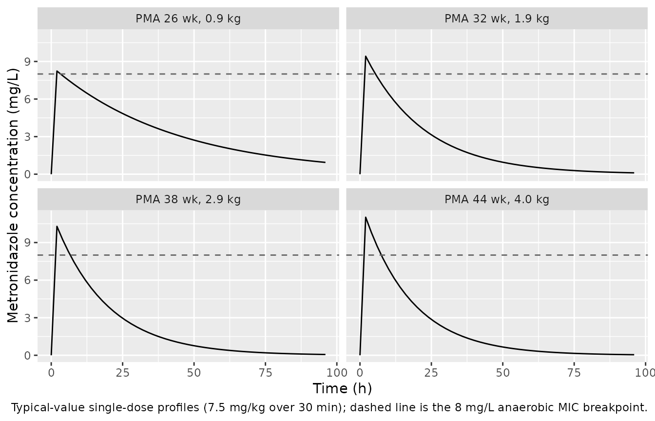
Prediction-corrected-style VPC of the PMA-based regimen (Figure 2)
Randell 2024 Figure 2 is a prediction-corrected VPC of the optimized model over the combined data set. The observed data are not public, so the panel below shows the simulated 5th / 50th / 95th percentiles from the packaged model under the guideline regimen; it reproduces the shape and level of the simulated band, not the overlaid observations.
sim |>
  dplyr::group_by(treatment, time) |>
  dplyr::summarise(
    Q05 = quantile(Cc, 0.05, na.rm = TRUE),
    Q50 = quantile(Cc, 0.50, na.rm = TRUE),
    Q95 = quantile(Cc, 0.95, na.rm = TRUE),
    .groups = "drop"
  ) |>
  dplyr::filter(time <= DOSE_END_H) |>
  ggplot(aes(time, Q50)) +
  geom_ribbon(aes(ymin = Q05, ymax = Q95), alpha = 0.25) +
  geom_line() +
  geom_hline(yintercept = 8, linetype = "dashed", colour = "grey40") +
  facet_wrap(~ factor(treatment, levels = ARM_LEVELS)) +
  labs(x = "Time (h)", y = "Metronidazole concentration (mg/L)",
       caption = "Simulated 5th / 50th / 95th percentiles, 150 virtual subjects per arm. Compare the first three panels with Figure 2 of Randell 2024; the fourth is the counterfactual described below.")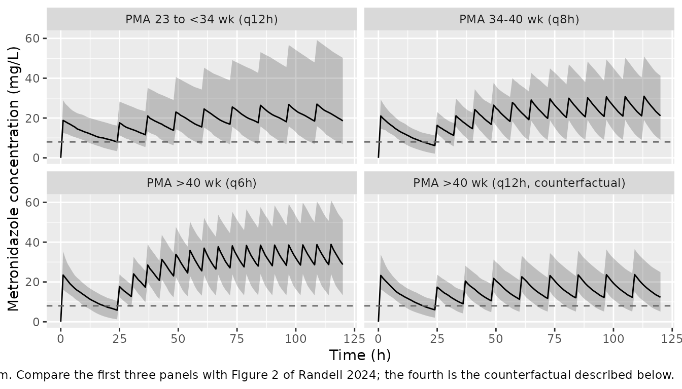
PKNCA validation
PKNCA computes steady-state Cmax, Cmin, Cavg and AUC over the last complete dosing interval of the simulated cohort, plus the terminal half-life on the post-dose washout.
tau_by_arm <- tibble::tibble(
  treatment = ARM_LEVELS,
  tau       = c(12, 8, 6, 12)
)

sim_nca <- sim |>
  dplyr::filter(!is.na(Cc)) |>
  dplyr::select(id, time, Cc, treatment) |>
  # Per subject, keep Cc >= 1e-6 * Cmax after the peak (and time zero): below that the ODE integrator has no relative accuracy left.
  dplyr::group_by(treatment, id) |>
  dplyr::filter(time == 0 | time <= time[which.max(Cc)] | Cc >= 1e-6 * max(Cc)) |>
  dplyr::ungroup() |>
  as.data.frame()

dose_df <- events |>
  dplyr::filter(evid == 1) |>
  dplyr::select(id, time, amt, treatment) |>
  as.data.frame()

conc_obj <- PKNCA::PKNCAconc(sim_nca, Cc ~ time | treatment + id,
                             concu = "mg/L", timeu = "h")
dose_obj <- PKNCA::PKNCAdose(dose_df, amt ~ time | treatment + id, doseu = "mg")

# Last complete dosing interval (steady state) per subject.
intervals_ss <- dose_df |>
  dplyr::group_by(treatment, id) |>
  dplyr::summarise(start = max(time), .groups = "drop") |>
  dplyr::left_join(tau_by_arm, by = "treatment") |>
  dplyr::mutate(end = start + tau, cmax = TRUE, cmin = TRUE,
                cav = TRUE, auclast = TRUE) |>
  dplyr::select(-tau) |>
  as.data.frame()

# Terminal decay after the last dose.
intervals_thalf <- dose_df |>
  dplyr::group_by(treatment, id) |>
  dplyr::summarise(start = max(time), .groups = "drop") |>
  dplyr::left_join(tau_by_arm, by = "treatment") |>
  dplyr::mutate(start = start + tau, end = Inf, half.life = TRUE) |>
  dplyr::select(-tau) |>
  as.data.frame()

intervals <- dplyr::bind_rows(intervals_ss, intervals_thalf) |>
  dplyr::mutate(dplyr::across(
    c(cmax, cmin, cav, auclast, half.life),
    ~ !is.na(.x) & .x
  ))

nca_res <- suppressWarnings(
  PKNCA::pk.nca(PKNCA::PKNCAdata(conc_obj, dose_obj, intervals = intervals))
)

res_tbl <- as.data.frame(nca_res$result)
Steady-state exposure by PMA band
ss_summary <- res_tbl |>
  dplyr::filter(PPTESTCD %in% c("cmax", "cmin", "cav", "auclast", "half.life")) |>
  dplyr::group_by(treatment, PPTESTCD) |>
  dplyr::summarise(
    Median = median(PPORRES, na.rm = TRUE),
    P05    = quantile(PPORRES, 0.05, na.rm = TRUE),
    P95    = quantile(PPORRES, 0.95, na.rm = TRUE),
    .groups = "drop"
  ) |>
  dplyr::mutate(PPTESTCD = factor(
    PPTESTCD,
    levels = c("cmax", "cmin", "cav", "auclast", "half.life"),
    labels = c("Cmax (mg/L)", "Cmin (mg/L)", "Cavg (mg/L)",
               "AUC(tau) (mg*h/L)", "Half-life (h)")
  )) |>
  dplyr::arrange(treatment, PPTESTCD) |>
  dplyr::rename("PMA band" = treatment, "NCA parameter" = PPTESTCD)

knitr::kable(ss_summary, digits = 2,
caption = "Simulated steady-state NCA parameters over the last dosing interval, and terminal half-life over the washout (median, 5th, 95th percentile; 150 virtual subjects per PMA band).")| PMA band | NCA parameter | Median | P05 | P95 |
|---|---|---|---|---|
| PMA 23 to <34 wk (q12h) | Cmax (mg/L) | 27.08 | 15.94 | 61.17 |
| PMA 23 to <34 wk (q12h) | Cmin (mg/L) | 18.57 | 6.89 | 50.24 |
| PMA 23 to <34 wk (q12h) | Cavg (mg/L) | 22.90 | 10.81 | 56.31 |
| PMA 23 to <34 wk (q12h) | AUC(tau) (mg*h/L) | 274.76 | 129.69 | 675.71 |
| PMA 23 to <34 wk (q12h) | Half-life (h) | 19.98 | 8.95 | 77.90 |
| PMA 34-40 wk (q8h) | Cmax (mg/L) | 31.01 | 19.08 | 51.39 |
| PMA 34-40 wk (q8h) | Cmin (mg/L) | 21.14 | 9.05 | 41.25 |
| PMA 34-40 wk (q8h) | Cavg (mg/L) | 25.71 | 13.25 | 45.73 |
| PMA 34-40 wk (q8h) | AUC(tau) (mg*h/L) | 205.67 | 105.99 | 365.84 |
| PMA 34-40 wk (q8h) | Half-life (h) | 13.61 | 6.47 | 26.63 |
| PMA >40 wk (q12h, counterfactual) | Cmax (mg/L) | 23.72 | 15.25 | 36.69 |
| PMA >40 wk (q12h, counterfactual) | Cmin (mg/L) | 12.31 | 5.15 | 24.90 |
| PMA >40 wk (q12h, counterfactual) | Cavg (mg/L) | 17.11 | 9.43 | 29.84 |
| PMA >40 wk (q12h, counterfactual) | AUC(tau) (mg*h/L) | 205.26 | 113.13 | 358.08 |
| PMA >40 wk (q12h, counterfactual) | Half-life (h) | 11.93 | 6.14 | 24.89 |
| PMA >40 wk (q6h) | Cmax (mg/L) | 38.94 | 24.01 | 61.42 |
| PMA >40 wk (q6h) | Cmin (mg/L) | 28.77 | 13.31 | 51.17 |
| PMA >40 wk (q6h) | Cavg (mg/L) | 33.43 | 17.39 | 55.79 |
| PMA >40 wk (q6h) | AUC(tau) (mg*h/L) | 200.58 | 104.34 | 334.72 |
| PMA >40 wk (q6h) | Half-life (h) | 11.16 | 4.98 | 22.13 |
Randell 2024 reports no NCA table, so there is no published Cmax /
AUC / half-life to place side by side here;
nlmixr2lib::ncaComparisonTable() is therefore not used. The
paper’s quantitative claims are its parameter estimates (checked in the
source trace and in Gates 1-3) and its dosing recommendation (checked
next).
The paper’s dosing conclusion
The stated conclusion is that the postmenstrual-age-based interval schedule “supports existing dosing guidelines” and “adds new data to support a 6-hour dosing interval for infants with postmenstrual age greater than 40 weeks”.
Two properties of the packaged model set up that conclusion, and both are exact consequences of the published equations rather than simulation artefacts.
Exposure per dose is weight-free. Because
CL = theta_CL * WT * fmat(PMA) is exactly linear in weight,
a mg/kg dose cancels the weight term:
AUC(tau) = Dose / CL = (7.5 * WT) / (0.036 * WT * fmat) = 208.3 / fmat mg*h/LGate 1 above shows this directly: the two fully mature typical subjects (2.9 kg and 4.0 kg) have AUC(tau) of 208.76 and 208.38 mg*h/L despite differing by 38 percent in weight. Weight-based dosing therefore fixes exposure per dose, and the only remaining choice is the interval.
Half-life falls as infants grow. V
scales as WT^0.763 while CL scales as
WT^1, so the elimination rate constant grows as
WT^0.237 and the half-life shrinks with size. The interval
must shorten to match.
thalf_by_arm <- res_tbl |>
  dplyr::filter(PPTESTCD == "half.life") |>
  dplyr::group_by(treatment) |>
  dplyr::summarise(median_thalf = median(PPORRES, na.rm = TRUE), .groups = "drop")

guideline_arms <- ARM_LEVELS[1:3]

thalf_guideline <- thalf_by_arm |>
  dplyr::filter(treatment %in% guideline_arms) |>
  dplyr::arrange(match(treatment, guideline_arms))

# Half-life must fall monotonically across the three guideline bands.
stopifnot(all(diff(thalf_guideline$median_thalf) < 0))
Median simulated half-life falls from 20.0 h in the youngest band to 13.6 h and 11.2 h in the two older bands.
The counterfactual. The question the paper answers for PMA above 40 weeks is whether the 12-hourly interval used in the youngest band would still cover those infants. The fourth simulated arm doses the >40 week cohort 12-hourly instead of 6-hourly.
exposure_by_arm <- dplyr::inner_join(
  res_tbl |>
    dplyr::filter(PPTESTCD == "cav") |>
    dplyr::group_by(treatment) |>
    dplyr::summarise(median_cav = median(PPORRES, na.rm = TRUE), .groups = "drop"),
  res_tbl |>
    dplyr::filter(PPTESTCD == "cmin") |>
    dplyr::group_by(treatment) |>
    dplyr::summarise(
      median_cmin        = median(PPORRES, na.rm = TRUE),
      pct_cmin_above_mic = 100 * mean(PPORRES > 8, na.rm = TRUE),
      .groups = "drop"
    ),
  by = "treatment"
) |>
  dplyr::arrange(match(treatment, ARM_LEVELS))

exposure_by_arm |>
  dplyr::rename(
    "Arm"                             = treatment,
    "Median Cavg (mg/L)"              = median_cav,
    "Median Cmin (mg/L)"              = median_cmin,
    "Subjects with Cmin > 8 mg/L (%)" = pct_cmin_above_mic
  ) |>
  knitr::kable(digits = 1,
caption = "Steady-state average and trough concentrations by arm, against the 8 mg/L anaerobic MIC breakpoint. The fourth arm is the counterfactual: the >40 week cohort dosed 12-hourly rather than 6-hourly.")| Arm | Median Cavg (mg/L) | Median Cmin (mg/L) | Subjects with Cmin > 8 mg/L (%) |
|---|---|---|---|
| PMA 23 to <34 wk (q12h) | 22.9 | 18.6 | 91.3 |
| PMA 34-40 wk (q8h) | 25.7 | 21.1 | 96.7 |
| PMA >40 wk (q6h) | 33.4 | 28.8 | 99.3 |
| PMA >40 wk (q12h, counterfactual) | 17.1 | 12.3 | 82.7 |
q6h  <- exposure_by_arm[exposure_by_arm$treatment == ARM_LEVELS[3], ]
q12h <- exposure_by_arm[exposure_by_arm$treatment == ARM_LEVELS[4], ]

trough_drop_pct  <- 100 * (q12h$median_cmin - q6h$median_cmin) / q6h$median_cmin
coverage_loss_pp <- q6h$pct_cmin_above_mic - q12h$pct_cmin_above_mic

# Every guideline band must keep the typical infant's trough above the MIC
# breakpoint, and the 6-hourly interval above 40 weeks PMA must do materially
# better than the 12-hourly counterfactual on both trough level and coverage.
stopifnot(
  all(exposure_by_arm$median_cmin[match(guideline_arms, exposure_by_arm$treatment)] > 8),
  trough_drop_pct  < -40,
  coverage_loss_pp > 10
)
Moving the >40 week cohort from 6-hourly to 12-hourly dosing drops the median steady-state trough by 57 percent and costs 17 percentage points of subjects holding a trough above the 8 mg/L breakpoint, while every guideline band keeps its typical infant above the breakpoint. That gap is the quantitative content of the paper’s recommendation to use a 6-hour interval above 40 weeks PMA.
Assumptions and deviations
-
The erratum supersedes the printed table.
hill_cl = 15.7comes from the 2025 erratum (doi:10.1128/aac.00972-25), not from the 2024 Table 1, which prints 7. The erratum states the typographical error “did not impact any modeling code or analysis”, so 15.7 is the value the published analysis actually used. -
Interindividual variability scale. Table 1 reports
IIV as %CV. The variances in
ini()use the log-normal relationomega^2 = log(CV^2 + 1)(0.11933 for CL, 0.06252 for V). If the authors instead reportedsqrt(omega^2) * 100, the variances would be 0.12674 and 0.06452 - a 6 and 3 percent difference in variance, respectively, which does not change any conclusion in this vignette. The paper does not reportomega^2on the raw scale, so the ambiguity cannot be resolved from the source. -
No reference weight or reference PMA. The published
equations are written on absolute body weight in kg
(
CL = theta_CL * WT,V = theta_V * WT^0.763) rather than on a weight ratio, sotheta_CLis a per-kg clearance andtheta_Vis the volume at 1 kg. No centering constant was introduced. -
PAGE unit conversion. The canonical covariate
PAGEis registered in months; the paper works in weeks.model()converts withpma_wk = PAGE * 4.35, so a user supplyingPAGEin months reproduces the published TM50 of 25.6 weeks exactly. - Virtual-cohort covariate distributions are assumed. The paper reports means and SDs, not joint distributions, for weight and PMA. The cohorts here draw weight and PMA independently from uniform ranges chosen to bracket the reported means within each PMA band; the real cohort’s weight and PMA are strongly correlated. This affects the width of the simulated percentile bands but not the typical-value gates, which are deterministic.
- Figure 2 is a shape comparison only. The observed concentrations that Figure 2 overlays are not public (data are available from the Pediatric Trials Network on request), so this vignette shows the simulated band without the observed percentiles.
-
Residual error is not applied to the simulated
summaries.
rxSolve()returnsCcas the individual prediction; the proportional residual error (19.1 percent) is a parameter of the model file but is not layered onto the NCA summaries, which therefore describe the underlying concentration-time course rather than the measured-with-error one. -
Supplemental Table S3 is an image. The
covariate-selection table in the supplement is supplied as a raster
image rather than text. The set of screened covariates recorded in
covariatesDataExcludedcomes from the Methods section (“Potential covariates including GA, PMA, postnatal age (PNA), sex, race, serum creatinine concentration, albumin concentration, and concomitant administration of the CYP3A inducer and/or CYP3A inhibitor”), which enumerates the same set. Race was screened but is not carried incovariatesDataExcludedbecause the paper does not state which race categories were tested. -
The PTN_METRO source model is not in this package.
The model this paper optimizes is Cohen-Wolkowiez 2013 (Pediatr Infect
Dis J 32:956-961, doi:10.1097/INF.0b013e3182947cf8), which is not
currently packaged. A different Cohen-Wolkowiez metronidazole model
built from scavenged samples is available as
CohenWolkowiez_2012_metronidazole; it is a related but distinct fit (power function of PMA on CL rather than a sigmoidal maturation function) and is not the PTN_METRO model.