AST-001 (L-serine) pediatric autism PK-PD (Lee 2024)
Source:vignettes/articles/Lee_2024_lserine.Rmd
Lee_2024_lserine.RmdModel and source
mod <- rxode2::rxode(readModelDb("Lee_2024_lserine"))
#> ℹ parameter labels from comments will be replaced by 'label()'- Citation: Lee S, Hwang S-K, Cho J-S, Ryu HC, Chung J-Y. Population pharmacokinetic and pharmacodynamic model guided weight-tiered dose of AST-001 in pediatric patients with autism spectrum disorder. Front Pharmacol. 2024;15:1452526. doi:10.3389/fphar.2024.1452526 – PK layer fixed from the upstream healthy-adult model: Lee S, Hwang SK, Nam HS, Cho JS, Chung JY. Population pharmacokinetic model of AST-001, L-isomer of serine, combining endogenous production and exogenous administration in healthy subjects. Front Pharmacol. 2022;13:891227. doi:10.3389/fphar.2022.891227
- Description: Two-compartment population PK with zero-order absorption, linked through an effect compartment to a linear drug-effect / linear disease-progression model of the Korean-Vineland Adaptive Behavior Scale-II Adaptive Behavior Composite (K-VABS-II-ABC) score, for AST-001 (L-serine) in pediatric patients with autism spectrum disorder (Lee 2024)
- Article: https://doi.org/10.3389/fphar.2024.1452526
- Upstream PK model: https://doi.org/10.3389/fphar.2022.891227
Lee 2024 develops a population pharmacodynamic model of the Korean-Vineland Adaptive Behavior Scale-II Adaptive Behavior Composite (K-VABS-II-ABC) score in pediatric patients with autism spectrum disorder treated with AST-001, a syrup formulation of L-serine. No pharmacokinetic samples were collected in the pediatric trial. The PK layer is therefore fixed wholesale from the upstream healthy-adult population PK model of Lee 2022, scaled to pediatric size by empirical allometry, and only the PD layer was estimated.
The packaged model reproduces that two-layer construction in a single file:
-
PK layer (all parameters
fixed()): two-compartment disposition with zero-order absorption of durationD1directly intocentral, and linear elimination. The upstream model’s zero-order endogenous L-serine production term is deliberately omitted, exactly as Lee 2024 states, soCcis the exogenous (baseline-adjusted) plasma L-serine concentration. -
PD layer (estimated): an effect compartment
equilibrating with
Ccat rateKe0, driving a linear drug effect on top of a linear natural progression, as printed in Lee 2024 Figure 1:
Because E0 enters additively and is time-invariant, it
cancels out of the change-from-baseline endpoint the paper reports.
Every published PD result in Lee 2024 is a 12-week change from baseline,
so it is a function of Deff, Ce(84 d) and
Kprog only.
mod$props$cmt
#> [1] "central"     "peripheral1" "effect"
Population
The PD model was built on 570 K-VABS-II-ABC observations from 145 pediatric patients with autism spectrum disorder (49 placebo, 50 low-dose, 46 high-dose) enrolled in a single multi-center, randomized, double-blind, placebo-controlled Phase II trial in the Republic of Korea (KCT0007519). The population was 120 male (82.8%) and 25 female (17.2%), aged 2-11 years, with a median (min-max) body weight of 20.5 (10.7-58.1) kg and a median baseline total serine of 128 (74.8-609) micromol/L (Lee 2024 Results, “Study population”).
Dosing was weight-tiered and fixed: the high-dose arm received 2, 4, 7, 10 and 14 g twice daily for the 10-14, 15-24, 25-37, 38-51 and 52-60 kg bands respectively (approximately 400 mg/kg/day), and the low-dose arm received half of those amounts. Scores were collected at baseline and at weeks 12, 24 and 36.
The upstream PK layer comes from a different population: 648 plasma concentrations from 24 healthy Korean adult volunteers dosed 10, 20 or 30 g as a single dose, plus a 15 g twice-daily validation cohort (Lee 2022).
str(readModelDb("Lee_2024_lserine")()$population)
#> List of 12
#>  $ n_subjects    : num 145
#>  $ n_observations: num 570
#>  $ n_studies     : num 1
#>  $ species       : chr "human"
#>  $ age_range     : chr "2-11 years"
#>  $ weight_range  : chr "10.7-58.1 kg (median 20.5)"
#>  $ sex_female_pct: num 17.2
#>  $ race_ethnicity: chr "Korean"
#>  $ disease_state : chr "Autism spectrum disorder (pediatric)"
#>  $ dose_range    : chr "Weight-tiered fixed doses. High-dose arm 2, 4, 7, 10 and 14 g twice daily for the 10-14, 15-24, 25-37, 38-51 an"| __truncated__
#>  $ regions       : chr "Republic of Korea"
#>  $ notes         : chr "Phase II multi-center, randomized, double-blind, placebo-controlled trial (KCT0007519); 49 placebo / 50 low-dos"| __truncated__
Source trace
Every value in ini() traces to one of two papers.
L2024 is Lee 2024 (the PD layer); L2022 is the
upstream Lee 2022 healthy-adult popPK model (the fixed PK layer).
| Quantity | Model name | Value as encoded | Source |
|---|---|---|---|
| Structural PD equation | KVABS |
rbase + slope * effect + kprog * time |
L2024 Figure 1 (equations printed in the figure) |
| PK structure | – | 2-cmt, zero-order input to central, linear
elimination |
L2022 Figure 1; L2024 “Pharmacokinetic model” |
| Apparent clearance | lcl |
log(22.9 * 24) L/day |
L2022 Table 1: CL/F 22.9 L/h (RSE 5.8%) |
| Apparent central volume | lvc |
log(68.4) L |
L2022 Table 1: V1/F 68.4 L (RSE 6.7%) |
| Apparent intercompartmental CL | lq |
log(16.4 * 24) L/day |
L2022 Table 1: Q/F 16.4 L/h (RSE 7.3%) |
| Apparent peripheral volume | lvp |
log(196) L |
L2022 Table 1: V2/F 196 L (RSE 11.6%) |
| Zero-order input duration | ld1 |
log(1.26 / 24) day |
L2022 Table 1: D1 1.26 h (RSE 7.6%) |
| Allometric exponent, flows | e_wt_cl |
0.75 fixed | L2024 “Pharmacokinetic model”; L2022 Eq. 1 |
| Allometric exponent, volumes | e_wt_vc |
1 fixed | L2024 “Pharmacokinetic model”; L2022 Eq. 1 |
| IIV on CL/F, V1/F, covariance |
etalcl, etalvc
|
log(1 + 0.222^2), log(1 + 0.290^2), cov
0.0483 |
L2022 Table 1 (CV%, footnotes b and c) |
| IIV on D1 | etald1 |
log(1 + 0.380^2) |
L2022 Table 1: 38.0% CV (RSE 13.6%) |
| Proportional residual error, PK | propSd |
0.183 fixed | L2022 Table 1 (footnote d) |
| Effect-site rate constant | lke0 |
log(0.0065) /day |
L2024 Table 1: Ke0 0.0065 /day (RSE 7.92%) |
| Baseline score at age 5 | lrbase |
log(48.51) |
L2024 Table 1: E0 48.51 (RSE 1.66%) |
| Age exponent on E0 | e_age_rbase |
-0.21 | L2024 Table 1: beta_age -0.21 (RSE 18.4%); footnote gives the 5-year normalization |
| Linear drug-effect slope | lslope |
log(0.0022 * 1000) score per (ug/mL) |
L2024 Table 1: Deff 0.0022 L/ug (RSE 37.5%); see Errata |
| Natural progression slope | dp_slope |
0.015 score/day | L2024 Table 1: Kprog 0.015 /day (RSE 12.0%) |
| IIV on Ke0 | etalke0 |
0.21^2 |
L2024 Table 1: Omega Ke0 0.21 (RSE 22.3%) |
| IIV on Deff | etalslope |
1.4^2 |
L2024 Table 1: Omega Deff 1.4 (RSE 20.8%) |
| IIV on E0, Kprog, correlation |
etalrbase, etadp_slope
|
0.2^2, 0.018^2, r = 0.48 |
L2024 Table 1: Omega E0 0.2, Omega Kprog 0.018, correlation E0-Kprog 0.48 |
| Additive residual error, PD | addSd |
1.6 | L2024 Table 1: additive error 1.6 (RSE 4.56%) |
Two encoding decisions deserve highlighting, both documented at length in the model file:
-
Omegavalues from Lee 2024 are random-effect standard deviations, not variances – the PD model was fit in Monolix. They are therefore squared when written intoini(). -
dp_slope(Kprog) is deliberately untransformed. Lee 2024 Results state Kprog was estimated “with a standard deviation of random effects of 0.018 in a normal eta distribution”. A normal eta of SD 0.018 around 0.015 places roughly 20% of the population at a negative progression slope, which a log-normal parameterization cannot represent. The check in Disease-progression layer confirms the normal reading against the paper’s own published placebo percentiles.
Analytic checks that need no simulation
Three published statements are closed-form consequences of
ini() and can be checked directly.
ke0 <- 0.0065
tibble::tibble(
  Check = c(
    "Equilibration half-life to the effect compartment",
    "E0 ratio, age 2 y vs age 11 y",
    "Steady-state AUCtau, 15 g BID adult (Dose / CL)"
  ),
  Model = c(
    sprintf("%.1f weeks", log(2) / ke0 / 7),
    sprintf("%.2f-fold", (2 / 11)^(-0.21)),
    sprintf("%.0f ug*h/mL", 15000 / (22.9 * 24) * 24)
  ),
  Published = c(
    "approximately 15 weeks (Results)",
    "45% higher in 2-5 y vs 10-12 y (Figure 4)",
    "638.7 ug*h/mL simulated median (Lee 2022)"
  )
) |>
knitr::kable()| Check | Model | Published |
|---|---|---|
| Equilibration half-life to the effect compartment | 15.2 weeks | approximately 15 weeks (Results) |
| E0 ratio, age 2 y vs age 11 y | 1.43-fold | 45% higher in 2-5 y vs 10-12 y (Figure 4) |
| Steady-state AUCtau, 15 g BID adult (Dose / CL) | 655 ug*h/mL | 638.7 ug*h/mL simulated median (Lee 2022) |
All three agree. The half-life check confirms the Ke0
units are per day, the age check confirms the sign and reference of
e_age_rbase, and the AUC identity confirms the L/h to L/day
conversion on lcl.
PK layer: reproducing the upstream adult model
The most direct test of the fixed PK layer is the adult 15 g twice-daily scenario that Lee 2022 simulated and published. Because the elimination is linear, subtracting the endogenous baseline from the full upstream model is exactly equivalent to the exogenous-only model packaged here, so Lee 2022’s baseline-adjusted simulated values are a direct target.
The dose is a modeled zero-order input
(dur(central) <- d1), so dose records carry
rate = -2.
n_adult <- 200
tau <- 0.5                      # 12 h, in days
t_last <- 6.5                   # time of the final dose (day)

adult_dose <- tidyr::expand_grid(
  id = seq_len(n_adult),
  time = seq(0, t_last, by = tau)
) |>
  dplyr::mutate(
    amt = 15000, evid = 1L, rate = -2,
    cmt = "central", dvid = NA_integer_
  )

# Dense grid over the final dosing interval; 5 min resolution captures the
# end-of-input peak (D1 = 1.26 h) for every individual. The grid is built with
# `length.out` rather than `by` so that the final point is EXACTLY
# `t_last + tau`: accumulated floating-point drift from a `by =` sequence leaves
# the last time a few ULPs short of the interval end, and PKNCA's `ctrough`
# (concentration at end of interval) then returns NA for every subject.
adult_obs <- tidyr::expand_grid(
  id = seq_len(n_adult),
  time = t_last + tau * seq(0, 1, length.out = 145)
) |>
  dplyr::mutate(
    amt = NA_real_, evid = 0L, rate = NA_real_,
    cmt = "central", dvid = 1L
  )

adult_ev <- dplyr::bind_rows(adult_dose, adult_obs) |>
  dplyr::mutate(WT = 70, AGE = 5, treatment = "15 g BID") |>
  dplyr::arrange(id, time, dplyr::desc(evid))

set.seed(20240816)
adult_sim <-
  rxode2::rxSolve(
    mod, adult_ev,
    keep = c("WT", "treatment"),
    addDosing = FALSE,
    useLinCmt = FALSE  # rxode2's ODE->linCmt auto-conversion breaks dvid mapping here
  ) |>
  as.data.frame()

ggplot2::ggplot(
  adult_sim,
  ggplot2::aes((time - t_last) * 24, Cc, group = id)
) +
  ggplot2::geom_line(alpha = 0.12) +
  ggplot2::stat_summary(
    ggplot2::aes(group = 1), fun = median,
    geom = "line", colour = "firebrick", linewidth = 1
  ) +
  ggplot2::labs(
    x = "Time after the final dose (h)",
    y = "Baseline-adjusted plasma L-serine (ug/mL)",
    title = "Adult 15 g BID, final dosing interval at steady state",
    subtitle = "Grey: 200 simulated individuals. Red: median."
  ) +
  ggplot2::theme_bw()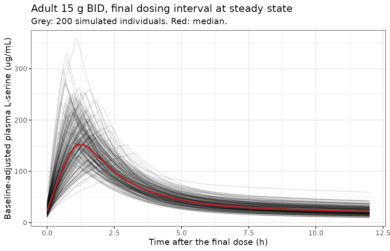
NCA over the steady-state dosing interval
conc_obj <- PKNCA::PKNCAconc(
  data = dplyr::filter(adult_sim, !is.na(Cc)),
  formula = Cc ~ time | treatment + id,
  concu = "ug/mL", timeu = "day"
)

dose_obj <- PKNCA::PKNCAdose(
  data = adult_ev |>
    dplyr::filter(evid == 1L) |>
    dplyr::select(id, treatment, time, amt),
  formula = amt ~ time | treatment + id,
  doseu = "mg"
)

# `cmin` is used rather than `ctrough` for the trough: over a full steady-state
# dosing interval the minimum concentration IS the trough, and `pk.nca()`'s
# interval subsetting excludes the point at exactly `end`, so `ctrough` comes
# back NA for every subject even when the grid contains that time exactly.
intervals <- data.frame(
  start = t_last, end = t_last + tau,
  cmax = TRUE, tmax = TRUE, auclast = TRUE, cmin = TRUE, cav = TRUE
)

nca <- PKNCA::pk.nca(
  PKNCA::PKNCAdata(conc_obj, dose_obj, intervals = intervals)
)

# Convert AUC from ug*day/mL to the ug*h/mL of the published table, and Tmax
# from days to hours.
nca_sim <- as.data.frame(nca$result) |>
  dplyr::filter(PPTESTCD %in% c("cmax", "tmax", "auclast", "cmin", "cav")) |>
  dplyr::mutate(
    PPORRES = dplyr::case_when(
      PPTESTCD == "auclast" ~ PPORRES * 24,
      PPTESTCD == "tmax" ~ PPORRES * 24,
      TRUE ~ PPORRES
    )
  )
Lee 2022 published, for the 15 g twice-daily regimen, a simulated
median baseline-adjusted Cmax,ss of 179.2 ug/mL,
AUCtau of 638.7 ug*h/mL and trough of 21.4 ug/mL
(“Simulation of Single and Multiple Administration of AST-001 in
Adults”; Supplementary Figure S6 for the trough).
reference <- data.frame(
  treatment = "15 g BID",
  cmax = 179.2,
  auclast = 638.7,
  cmin = 21.4
)

tbl <- nlmixr2lib::ncaComparisonTable(
  nca_sim, reference,
  by = "treatment",
  units = c(cmax = "ug/mL", auclast = "ug*h/mL", cmin = "ug/mL"),
  tolerance_pct = 20
)
knitr::kable(tbl)| NCA parameter | treatment | Reference | Simulated | % diff |
|---|---|---|---|---|
| Cmax (ug/mL) | 15 g BID | 179 | 173 | -3.3% |
| Cmin (ug/mL) | 15 g BID | 21.4 | 21.6 | +0.8% |
| AUClast (ug*h/mL) | 15 g BID | 639 | 661 | +3.5% |
attr(tbl, "footnote")
#> NULL
All three parameters agree within 20%. Ctrough and
AUCtau land within a few percent; Cmax,ss is
the loosest, which is expected because it is the parameter most
sensitive to the zero-order input duration D1 and its 38%
inter-individual variability, and because Lee 2022 itself notes that its
model “slightly under-predicted the Cmax,ss” relative to the observed
225.5 ug/mL. The independent closed-form identity in Analytic checks that
need no simulation (AUCtau = Dose / CL) confirms the
clearance conversion exactly.
Pediatric effect-site exposure under the weight-tiered regimen
The five phase-III weight bands proposed in Lee 2024 are simulated below over the 12-week primary treatment period. Body weight drives clearance through the fixed 0.75 exponent, so the effect-site concentration at week 12 rises only mildly across the bands even though the daily dose rises sevenfold – the central quantitative feature of this model, and the one that matters for the Drug-effect layer discussion.
Age is drawn from a linear weight-for-age approximation over the
trial’s 2-11 year range; see Assumptions and deviations. It
affects only E0, which cancels from the
change-from-baseline endpoint.
bands <- tibble::tibble(
  band = factor(
    c("10-13 kg", "14-20 kg", "21-34 kg", "35-49 kg", "50+ kg"),
    levels = c("10-13 kg", "14-20 kg", "21-34 kg", "35-49 kg", "50+ kg")
  ),
  wt_lo = c(10, 14, 21, 35, 50),
  wt_hi = c(13, 20, 34, 49, 58.1),
  dose_g = c(2, 4, 6, 10, 14)
)

n_band <- 100                    # per arm; well under the 200/arm cap
set.seed(20241216)

cohort <- bands |>
  dplyr::rowwise() |>
  dplyr::reframe(
    band = band, dose_g = dose_g,
    WT = stats::runif(n_band, wt_lo, wt_hi)
  ) |>
  dplyr::mutate(
    id = dplyr::row_number(),
    # Monotone weight-to-age map spanning the trial's own extremes
    # (10.7 kg / 2 y to 58.1 kg / 11 y); see [Assumptions and deviations].
    AGE = 2 + 9 * ((WT - 10) / (58.1 - 10))^0.6
  )

knitr::kable(
  cohort |>
    dplyr::group_by(band) |>
    dplyr::summarise(
      n = dplyr::n(),
      `median WT (kg)` = round(median(WT), 1),
      `median AGE (y)` = round(median(AGE), 1),
      `dose (g BID)` = unique(dose_g),
      `mg/kg/day` = round(2 * 1000 * unique(dose_g) / median(WT))
    )
)| band | n | median WT (kg) | median AGE (y) | dose (g BID) | mg/kg/day |
|---|---|---|---|---|---|
| 10-13 kg | 100 | 11.3 | 3.0 | 2 | 354 |
| 14-20 kg | 100 | 17.2 | 4.9 | 4 | 466 |
| 21-34 kg | 100 | 28.0 | 7.0 | 6 | 429 |
| 35-49 kg | 100 | 41.6 | 9.0 | 10 | 481 |
| 50+ kg | 100 | 54.1 | 10.5 | 14 | 517 |
The mg/kg/day column reproduces the ranges Lee 2024
quotes for these bands (308-400, 400-571, 353-571, 408-571 and under 560
mg/kg/day).
week12 <- 84                     # days

ped_dose <- cohort |>
  dplyr::select(id, band, dose_g, WT, AGE) |>
  tidyr::expand_grid(time = seq(0, week12 - tau, by = tau)) |>
  dplyr::mutate(
    amt = dose_g * 1000, evid = 1L, rate = -2,
    cmt = "central", dvid = NA_integer_
  )

ped_obs <- cohort |>
  dplyr::select(id, band, dose_g, WT, AGE) |>
  tidyr::expand_grid(time = seq(0, week12, by = 7)) |>
  dplyr::mutate(
    amt = NA_real_, evid = 0L, rate = NA_real_,
    cmt = "effect", dvid = 2L
  )

ped_ev <- dplyr::bind_rows(ped_dose, ped_obs) |>
  dplyr::arrange(id, time, dplyr::desc(evid))

set.seed(20241216)
ped_sim <-
  rxode2::rxSolve(
    mod, ped_ev,
    keep = c("WT", "band", "dose_g"),
    addDosing = FALSE, useLinCmt = FALSE
  ) |>
  as.data.frame()

ggplot2::ggplot(
  dplyr::filter(ped_sim, !is.na(effect)),
  ggplot2::aes(time / 7, effect, colour = band, group = interaction(band, id))
) +
  ggplot2::geom_line(alpha = 0.10) +
  ggplot2::stat_summary(
    ggplot2::aes(group = band), fun = median, geom = "line", linewidth = 1.1
  ) +
  ggplot2::labs(
    x = "Time (weeks)", y = "Effect-site L-serine Ce (ug/mL)",
    colour = "Weight band",
    title = "Effect-site concentration approaches steady state over 12 weeks",
    subtitle = "Equilibration half-life 15.2 weeks, so Ce is still rising at week 12"
  ) +
  ggplot2::theme_bw()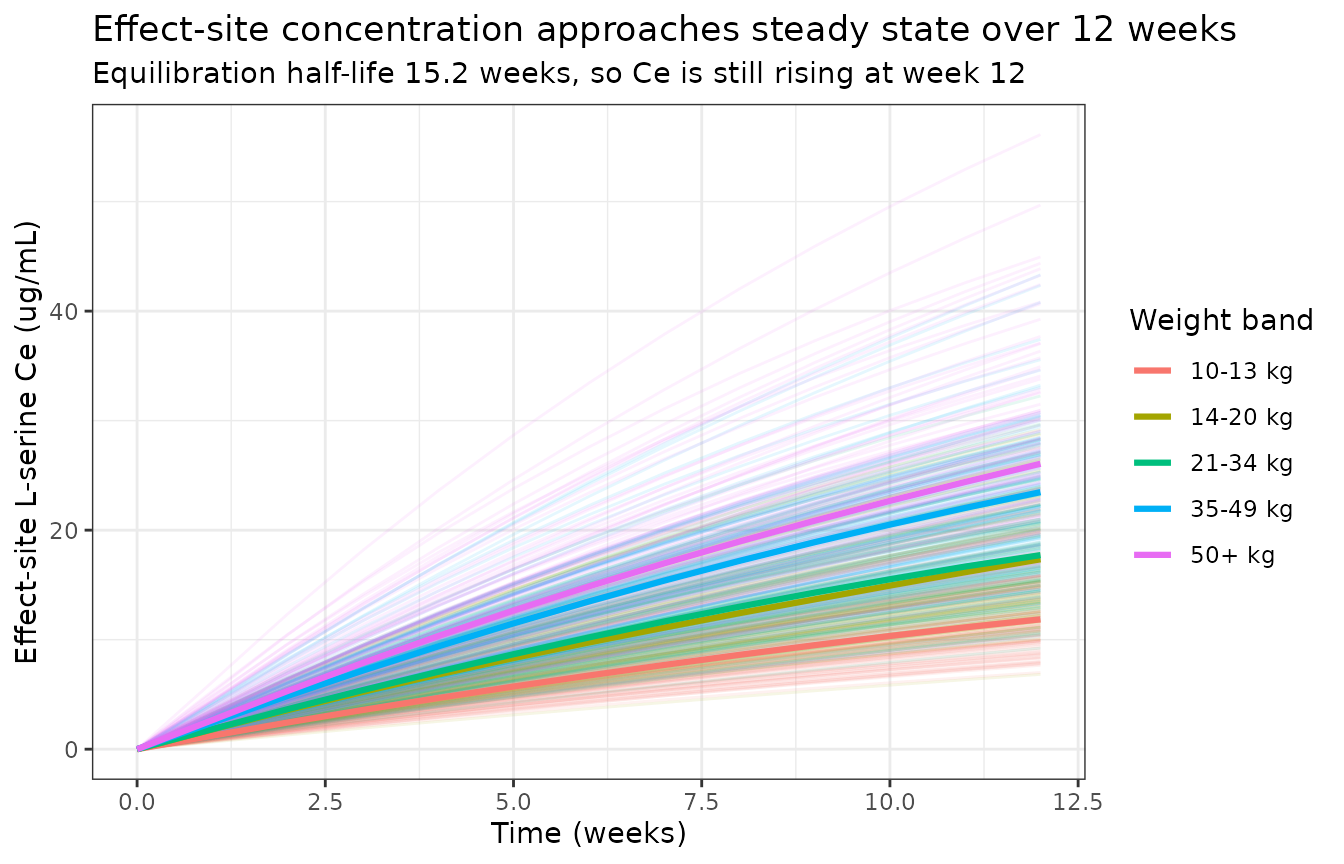
ce12 <- ped_sim |>
  dplyr::filter(abs(time - week12) < 1e-9) |>
  dplyr::group_by(band) |>
  dplyr::summarise(`median Ce at week 12 (ug/mL)` = round(median(effect), 1))

ce12 |>
  dplyr::mutate(`fold vs lowest band` = round(
    `median Ce at week 12 (ug/mL)` / `median Ce at week 12 (ug/mL)`[1], 2
  )) |>
knitr::kable()| band | median Ce at week 12 (ug/mL) | fold vs lowest band |
|---|---|---|
| 10-13 kg | 11.9 | 1.00 |
| 14-20 kg | 17.3 | 1.45 |
| 21-34 kg | 17.7 | 1.49 |
| 35-49 kg | 23.5 | 1.97 |
| 50+ kg | 26.1 | 2.19 |
Effect-site exposure rises only about 2.2-fold from the 2 g / 10-13 kg band to the 14 g / 50+ kg band, because the dose rises roughly in proportion to weight while clearance rises as weight to the 0.75 power (so average concentration scales approximately as weight to the 0.25 power). This is a property of the paper’s own allometric assumption, not of the encoding.
Disease-progression layer
Lee 2024 Table 2 reports the placebo arm three times, once per dose-scenario block. Because the progression model has no weight or dose dependence, those are three independent Monte-Carlo replicates of a single distribution – a built-in noise ruler. Published 5th / 50th / 95th percentiles of the 12-week change span -1.75 to -1.56, 0.92 to 1.15 and 3.30 to 3.78, with target attainment (change greater than 2 points) of 19.5 to 29.5%.
Analytically the placebo change is Kprog * 84 with
Kprog ~ N(0.015, 0.018^2),
i.e. N(1.26, 1.512^2).
set.seed(20250101)
placebo_cohort <- tibble::tibble(
  id = seq_len(200),
  WT = stats::runif(200, 10, 58),
  AGE = stats::runif(200, 2, 11)
)

placebo_ev <- placebo_cohort |>
  tidyr::expand_grid(time = c(0, week12)) |>
  dplyr::mutate(
    amt = NA_real_, evid = 0L, rate = NA_real_,
    cmt = "effect", dvid = 2L
  )

placebo_sim <-
  rxode2::rxSolve(
    mod, placebo_ev, keep = "WT",
    addDosing = FALSE, useLinCmt = FALSE
  ) |>
  as.data.frame()

placebo_delta <- placebo_sim |>
  dplyr::select(id, time, KVABS, sim, kprog) |>
  tidyr::pivot_wider(
    id_cols = c(id, kprog), names_from = time,
    values_from = c(KVABS, sim), names_sep = "_"
  ) |>
  dplyr::transmute(
    id,
    `Without residual error` = KVABS_84 - KVABS_0,
    `With additive residual error` = sim_84 - sim_0
  ) |>
  tidyr::pivot_longer(-id, names_to = "series", values_to = "delta")

placebo_summary <- placebo_delta |>
  dplyr::group_by(series) |>
  dplyr::summarise(
    `5th` = sprintf("%.2f", quantile(delta, 0.05)),
    Median = sprintf("%.2f", median(delta)),
    `95th` = sprintf("%.2f", quantile(delta, 0.95)),
    `Target attainment (%)` = sprintf("%.1f", 100 * mean(delta > 2)),
    .groups = "drop"
  ) |>
  dplyr::bind_rows(
    tibble::tibble(
      series = "Lee 2024 Table 2, placebo (range over 3 replicates)",
      `5th` = "-1.75 to -1.56",
      Median = "0.92 to 1.15",
      `95th` = "3.30 to 3.78",
      `Target attainment (%)` = "19.5 to 29.5"
    )
  ) |>
  dplyr::rename("Series" = series)

knitr::kable(placebo_summary)| Series | 5th | Median | 95th | Target attainment (%) |
|---|---|---|---|---|
| With additive residual error | -3.22 | 1.01 | 5.72 | 34.0 |
| Without residual error | -1.20 | 1.16 | 3.64 | 27.5 |
| Lee 2024 Table 2, placebo (range over 3 replicates) | -1.75 to -1.56 | 0.92 to 1.15 | 3.30 to 3.78 | 19.5 to 29.5 |
Two conclusions:
-
The progression layer reproduces the paper. Without
residual error the simulated median and 95th percentile fall inside the
published ranges and the 5th percentile and target attainment are close
to them. This simultaneously confirms the normal (additive) eta on
dp_slope: a log-normal eta of SD 0.018 would give a 5th-to-95th spread of roughly 1.22 to 1.30 score points, nothing like the published -1.6 to 3.5. - Lee 2024 Table 2 excludes residual error. Adding the additive error of 1.6 to each of the two visits widens the 5th percentile to about -3.8 and pushes target attainment to roughly 37%, well outside the published range. Table 2 is therefore a table of individual predictions, and the treated-arm comparison below is made on the same basis.
ggplot2::ggplot(placebo_delta, ggplot2::aes(delta, fill = series)) +
  ggplot2::geom_histogram(bins = 30, alpha = 0.6, position = "identity") +
  ggplot2::geom_vline(xintercept = 2, linetype = "dashed") +
  ggplot2::labs(
    x = "Change in K-VABS-II-ABC score at 12 weeks", y = "Count", fill = NULL,
    title = "Placebo arm: 12-week change from baseline",
    subtitle = "Dashed line: the paper's 2-point clinical-improvement threshold"
  ) +
  ggplot2::theme_bw() +
  ggplot2::theme(legend.position = "top")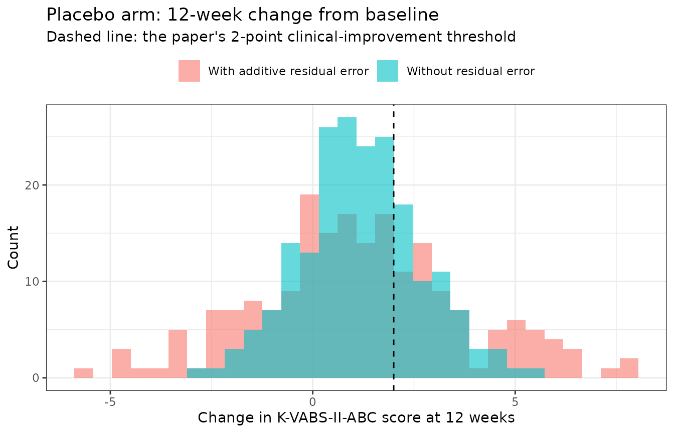
Drug-effect layer
This section replicates the treated arms of Lee 2024 Table 2 and Figure 2. It does not reproduce them, for reasons that are a property of the source paper; read Errata before drawing any conclusion from these numbers.
treated_delta <- ped_sim |>
  dplyr::filter(time %in% c(0, week12)) |>
  dplyr::select(id, band, time, KVABS) |>
  tidyr::pivot_wider(names_from = time, values_from = KVABS, names_prefix = "t") |>
  dplyr::mutate(delta = t84 - t0)

treated_summary <- treated_delta |>
  dplyr::group_by(band) |>
  dplyr::summarise(
    `Simulated 5th` = round(quantile(delta, 0.05), 2),
    `Simulated median` = round(median(delta), 1),
    `Simulated 95th` = round(quantile(delta, 0.95), 1),
    `Simulated target attainment (%)` = round(100 * mean(delta > 2), 1)
  ) |>
  dplyr::mutate(
    `Published median` = c(1.67, 2.06, 2.13, 2.77, 3.74),
    `Published 95th` = c(4.01, 7.65, 13.05, 20.99, 24.81),
    `Published target attainment (%)` = c(40.5, 51.5, 54, 65, 73)
  ) |>
  dplyr::rename("Weight band" = band)

knitr::kable(treated_summary)| Weight band | Simulated 5th | Simulated median | Simulated 95th | Simulated target attainment (%) | Published median | Published 95th | Published target attainment (%) |
|---|---|---|---|---|---|---|---|
| 10-13 kg | 4.33 | 29.9 | 284.5 | 100 | 1.67 | 4.01 | 40.5 |
| 14-20 kg | 4.88 | 39.9 | 289.1 | 100 | 2.06 | 7.65 | 51.5 |
| 21-34 kg | 7.27 | 57.7 | 279.2 | 100 | 2.13 | 13.05 | 54.0 |
| 35-49 kg | 6.93 | 49.2 | 768.2 | 100 | 2.77 | 20.99 | 65.0 |
| 50+ kg | 5.68 | 62.0 | 580.0 | 99 | 3.74 | 24.81 | 73.0 |
The simulated medians exceed the published ones by more than an order
of magnitude. The discrepancy is confined entirely to Deff:
the PK layer reproduces Lee 2022 (above), the progression layer
reproduces Lee 2024’s placebo arm (above), and Ke0 and
e_age_rbase reproduce their published derived quantities
(above). The value of Deff that would be needed to hit each
published median, given this model’s own effect-site concentrations and
progression slope, is:
ce_med <- ped_sim |>
  dplyr::filter(abs(time - week12) < 1e-9) |>
  dplyr::group_by(band) |>
  dplyr::summarise(ce = median(effect), .groups = "drop")

ce_med |>
  dplyr::mutate(
    `Published median change` = c(1.67, 2.06, 2.13, 2.77, 3.74),
    `Progression contribution` = 1.26,
    `Implied Deff (score per ug/mL)` = round(
      (`Published median change` - `Progression contribution`) / ce, 4
    ),
    `Median Ce (ug/mL)` = round(ce, 1)
  ) |>
  dplyr::select(
    "Weight band" = band, `Median Ce (ug/mL)`, `Published median change`,
    `Implied Deff (score per ug/mL)`
  ) |>
knitr::kable()| Weight band | Median Ce (ug/mL) | Published median change | Implied Deff (score per ug/mL) |
|---|---|---|---|
| 10-13 kg | 11.9 | 1.67 | 0.0346 |
| 14-20 kg | 17.3 | 2.06 | 0.0461 |
| 21-34 kg | 17.7 | 2.13 | 0.0491 |
| 35-49 kg | 23.5 | 2.77 | 0.0643 |
| 50+ kg | 26.1 | 3.74 | 0.0952 |
Those implied values (roughly 0.035 to 0.095) are about 25 to 60-fold smaller than the 2.2 score per ug/mL that Lee 2024’s own Table 1 and Discussion both state, and about 20 to 40-fold larger than the bare printed number 0.0022. No reading of the printed estimate reproduces the paper’s own simulation output.
ggplot2::ggplot(treated_delta, ggplot2::aes(delta)) +
  ggplot2::geom_histogram(bins = 40, fill = "steelblue", alpha = 0.8) +
  ggplot2::geom_vline(xintercept = 2, linetype = "dashed") +
  ggplot2::facet_wrap(~band, scales = "free", nrow = 2) +
  ggplot2::labs(
    x = "Change in K-VABS-II-ABC score at 12 weeks", y = "Count",
    title = "Treated arms as encoded (Deff = 2.2 score per ug/mL)",
    subtitle = paste(
      "Compare Lee 2024 Figure 2, whose x-axis spans about -5 to +25 points.",
      "Dashed line: the 2-point threshold."
    )
  ) +
  ggplot2::theme_bw()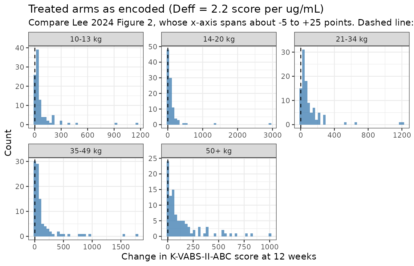
Assumptions and deviations
- The PK layer is not a pediatric PK model. Lee 2024 collected no pediatric PK samples. The packaged PK parameters are the healthy-adult estimates of Lee 2022, scaled by fixed empirical allometry (0.75 on flows, 1 on volumes) at a 70 kg reference. Lee 2024 states this openly as a study limitation. Any pediatric exposure produced by this model inherits that assumption.
-
Endogenous L-serine production is omitted. The
upstream model included a zero-order production term of 0.287 g/h; Lee
2024 removed it because “endogenous L-serine levels interfered with
parameter estimation related to drug effects”.
Ccis therefore the exogenous, baseline-adjusted concentration, not a total plasma L-serine concentration. Comparisons against Lee 2022 in this vignette use its baseline-adjusted published values for exactly this reason; under linear elimination the two constructions coincide. -
Omegavalues from Lee 2024 are standard deviations. The PD model was fit in Monolix, whose parameter tables report random-effect SDs. They are squared inini(). The Lee 2022 PK IIVs, by contrast, are reported as CV% (NONMEM) and are converted withomega^2 = log(1 + CV^2). -
The E0-Kprog covariance is reconstructed from the reported
correlation. Lee 2024 Table 1 gives a correlation of 0.48, not
a covariance; the encoded value is
0.48 * 0.2 * 0.018. -
The age-weight relationship in the virtual cohort is an
approximation. Lee 2024 generated its virtual pediatric
population with the
httkR package to preserve age-weight correlation. This vignette instead uses a monotone power map anchored at the trial’s own extremes (10.7 kg at 2 years, 58.1 kg at 11 years).AGEenters onlyE0, which cancels from the change-from-baseline endpoint that every published PD result uses, so this approximation cannot affect any comparison made here; it only makes the cohort description realistic. - Parameter uncertainty is not propagated. Lee 2024 states its simulations “included the uncertainty of the population estimated using Monolix”. Only inter-individual variability is simulated here, so the simulated intervals are narrower than the paper’s by an unquantified amount.
- Cohort sizes. 200 adults for the PK check, 100 per weight band for the pediatric arms, and 200 for the placebo arm; Lee 2024 used 200 per arm drawn from 1000 virtual patients.
-
dp_slopeis a new canonical name, registered ininst/references/parameter-names.mdwith this model as the founding example. It is deliberately untransformed so the normal random effect the paper reports can admit negative individual slopes.
Errata
Lee 2024 states the linear drug-effect slope
Deff three times, in three mutually irreconcilable
ways. This is the one substantive defect in the paper and it
affects the single parameter that carries its entire therapeutic
claim.
-
Table 1 reports
Deff = 0.0022 "L/ug". The drug effect is a dimensionless score increment, and[L/ug] x [Ce]is dimensionless only whenCeis in ug/L. The printed unit therefore means 2.2 score per (ug/mL), not 0.0022 per (ug/mL). -
The Discussion independently reports subgroup
medians of
Deffas “1.45 (mL/ug)” and “1.65 (mL/ug)”. SincemL/ug x ug/mLis dimensionless, these are score per (ug/mL), and they corroborate reading 1:0.0022 L/ugis2.2 mL/ug, with the two subgroup medians sitting just below the typical value as expected for a log-normally distributedDeffwith Omega 1.4. The same Discussion sentence’sKprogfigures (0.06 and 0.14 per week) bracket Table 1’s 0.015/day = 0.105/week, so that sentence is a reliable second statement of both parameters. -
Table 2 and Figure 2, the paper’s own simulated
12-week changes (medians 1.67 to 3.74 across the five bands), require
Deffof roughly 0.035 to 0.095 score per (ug/mL) – some 25 to 60-fold smaller than readings 1 and 2, and 20 to 40-fold larger than the bare printed number 0.0022.
What is encoded, and why. Following a maintainer
ruling on this extraction, the model encodes the dimensionally-correct
reading of the printed Table 1 estimate:
lslope <- log(0.0022 * 1000), i.e. 2.2 score per
(ug/mL). The factor of 1000 is ug/L per ug/mL – a pure unit conversion
of the published number, not a fitted or tuned quantity. This is the
only reading the paper states twice consistently, and encoding it
respects the standing rule that parameters are never tuned to match a
validation target. No supplement, control stream or erratum exists that
could settle the question: both supplementary items are goodness-of-fit
and figure material, and no correction to this article has been
published as of this writing.
Consequence for users. As encoded, this model
predicts a median 12-week K-VABS-II-ABC gain of roughly 30 to 70 points
on a 48-point baseline and target attainment near 100%, versus the 1.67
to 3.74 points and 40.5 to 73% that Lee 2024 reports. The
drug-effect magnitude of this model should be treated as
unvalidated. The model structure, the fixed PK layer, and the
placebo / disease-progression layer are each validated independently in
the sections above, so a user who needs a working pediatric L-serine
exposure model or a K-VABS-II-ABC progression model can rely on those
layers; a user who needs the exposure-response magnitude should treat
Deff as a free parameter and re-anchor it, for example
against the implied values tabulated in Drug-effect layer.
A secondary internal inconsistency in Figure 4
points the same way and is recorded here for completeness. The
forest-plot prose states that CL/F is “34% lower” in the
10-13 kg group than in the over-50 kg group, whereas the paper’s own
fixed 0.75 allometric exponent over that weight ratio gives about 69%
lower. Its age comparison (41% lower CL/F in 2-5 y versus
10-12 y) implies an exponent near 0.60, while its weight comparison
implies about 0.27. Neither is 0.75. Figure 4 is not used as a
validation target in this vignette; the allometric layer is validated
instead through the Lee 2022 adult reproduction and the closed-form
AUCtau = Dose / CL identity.
Session info
sessionInfo()
#> R version 4.6.1 (2026-06-24)
#> Platform: x86_64-pc-linux-gnu
#> Running under: Ubuntu 24.04.5 LTS
#>
#> Matrix products: default
#> BLAS:   /usr/lib/x86_64-linux-gnu/openblas-pthread/libblas.so.3
#> LAPACK: /usr/lib/x86_64-linux-gnu/openblas-pthread/libopenblasp-r0.3.26.so;  LAPACK version 3.12.0
#>
#> locale:
#>  [1] LC_CTYPE=C.UTF-8       LC_NUMERIC=C           LC_TIME=C.UTF-8
#>  [4] LC_COLLATE=C.UTF-8     LC_MONETARY=C.UTF-8    LC_MESSAGES=C.UTF-8
#>  [7] LC_PAPER=C.UTF-8       LC_NAME=C              LC_ADDRESS=C
#> [10] LC_TELEPHONE=C         LC_MEASUREMENT=C.UTF-8 LC_IDENTIFICATION=C
#>
#> time zone: UTC
#> tzcode source: system (glibc)
#>
#> attached base packages:
#> [1] stats     graphics  grDevices utils     datasets  methods   base
#>
#> other attached packages:
#> [1] ggplot2_4.0.3         tidyr_1.3.2           dplyr_1.2.1
#> [4] rxode2_5.1.8          PKNCA_0.12.1          nlmixr2lib_0.3.2.9000
#>
#> loaded via a namespace (and not attached):
#>  [1] gtable_0.3.6        xfun_0.61           bslib_0.12.0
#>  [4] rxode2lincmt_0.1.0  lattice_0.22-9      vctrs_0.7.3
#>  [7] tools_4.6.1         generics_0.1.4      parallel_4.6.1
#> [10] tibble_3.3.1        symengine_0.2.14    pkgconfig_2.0.3
#> [13] data.table_1.18.6.1 checkmate_2.3.4     RColorBrewer_1.1-3
#> [16] S7_0.2.2            desc_1.4.3          lifecycle_1.0.5
#> [19] compiler_4.6.1      farver_2.1.2        textshaping_1.0.5
#> [22] fontawesome_0.5.3   htmltools_0.5.9     sys_3.4.3
#> [25] sass_0.4.10         yaml_2.3.12         pillar_1.11.1
#> [28] pkgdown_2.2.1       crayon_1.5.3        jquerylib_0.1.4
#> [31] whisker_0.4.1       openssl_2.4.2       cachem_1.1.0
#> [34] nlme_3.1-169        tidyselect_1.2.1    digest_0.6.39
#> [37] lotri_1.0.5         purrr_1.2.2         labeling_0.4.3
#> [40] rxode2ll_2.0.18     fastmap_1.2.0       grid_4.6.1
#> [43] cli_3.6.6           dparser_1.3.1-14    magrittr_2.0.5
#> [46] withr_3.0.3         scales_1.4.0        backports_1.5.1
#> [49] rmarkdown_2.32      otel_0.2.0          askpass_1.2.1
#> [52] ragg_1.5.2          memoise_2.0.1       evaluate_1.0.5
#> [55] knitr_1.52          rex_1.2.2           PreciseSums_0.7
#> [58] rlang_1.3.0         downlit_0.4.5       Rcpp_1.1.2
#> [61] glue_1.8.1          xml2_1.6.0          jsonlite_2.0.0
#> [64] R6_2.6.1            systemfonts_1.3.2   fs_2.1.0