BHMA / alpha interferon in mice (Benson 2010)
Source:vignettes/articles/Benson_2010_bhma_mouse.Rmd
Benson_2010_bhma_mouse.RmdModel and source
- Citation: Benson N, de Jongh J, Duckworth JD, Jones HM, Pertinez HE, Rawal JK, van Steeg TJ, Van der Graaf PH. Pharmacokinetic-pharmacodynamic modeling of alpha interferon response induced by a Toll-like 7 receptor agonist in mice. Antimicrob Agents Chemother. 2010;54(3):1179-1185. doi:10.1128/AAC.00551-09
- Description: Preclinical (mouse, male CD-1 outbred). Sequential PK-PD model for the Toll-like receptor 7 (TLR-7) agonist BHMA [9-benzyl-8-hydroxy-2-(2-methoxyethoxy) adenine] with plasma alpha interferon (IFN-alpha) as the pharmacodynamic biomarker (Benson 2010). Stage 1: two-compartment apparent oral PK with first-order absorption (NONMEM ADVAN4), all disposition parameters reported per kilogram body weight; the absorption rate constant was fixed at 35 1/h because absorption was complete before the earliest PK sample at 0.1 h, and bioavailability could not be estimated without intravenous data, so CL, Vc, Q and Vp are apparent (/F) values. Stage 2: indirect-response (turnover) model for plasma IFN-alpha in which the drug STIMULATES synthesis through an ordinary Emax (non-sigmoid) function of the predicted plasma BHMA concentration and IFN-alpha is removed by a first-order rate constant, d(IFN)/dt = Smax * Cc / (SC50 + Cc) - kout * IFN. The IFN-alpha baseline is fixed at zero because unstimulated levels were below the 0.3 IU/mL assay LOQ in every animal. The Emax form beat a linear drug-effect alternative by dAIC = -22.9. Parameters from Benson 2010 Table 1 (PK) and Table 2 (PK-PD); no covariates were retained in either stage.
- Article: Antimicrob Agents Chemother 2010;54(3):1179-1185 (open access via PMC2825998)
Benson and colleagues dosed mice orally with the Toll-like receptor 7 (TLR-7) agonist BHMA – 9-benzyl-8-hydroxy-2-(2-methoxyethoxy) adenine – and measured both plasma BHMA and the induced plasma alpha interferon (IFN-alpha) response. TLR-7 agonists were being pursued as better-tolerated alternatives to recombinant IFN-alpha for hepatitis C, and the paper is the first published PK-PD model linking a TLR-7 agonist’s plasma exposure to the IFN-alpha biomarker it induces.
The model is sequential. Stage 1 is an apparent two-compartment oral
PK model (NONMEM ADVAN4). Stage 2 is an indirect-response (turnover)
model in which the predicted plasma BHMA concentration
stimulates the synthesis of IFN-alpha through an
ordinary Emax function, and IFN-alpha is removed by a first-order rate
constant. The IFN-alpha baseline is fixed at zero because unstimulated
levels were below the assay limit of quantification in every animal, so
the production term has no kin offset at all – the pool is
created entirely by drug.
Population
The study used male CD-1 outbred mice (Charles River Laboratories UK), healthy and uninfected. Two sets of animals contributed:
- PD groups (composite biomarker + PK sampling), dosed once orally at 0.1 mg/kg (n = 3), 0.3 mg/kg (n = 2), 0.5 mg/kg (n = 2), 1 mg/kg (n = 10), 2.5 mg/kg (n = 4), 5 mg/kg (n = 20) and 10 mg/kg (n = 5) – 46 animals.
- PK-only groups, dosed at 0.1, 1 and 5 mg/kg – 25 animals, sampled at 0.1, 0.25, 1, 2, 6, 8, 10 and 24 h (5 mg/kg) or 1, 2, 6, 8 and 10 h (1 and 0.1 mg/kg).
BHMA was given in 5% DMSO / 50% PEG-200 / 45% water. A matrix (composite) sampling design was used: two 50 uL saphenous-vein samples plus one terminal 1 mL sample per animal, so neither the PK nor the biomarker profile is fully serial within an animal. BHMA was quantified by LC-MS/MS (LOQ 0.5 ng/mL, assay CV 20%); IFN-alpha by a modified PBL Biomedical ELISA (LOQ 0.3 IU/mL, assay CV 20%), with 1 IU/mL taken to equal 15 pg/mL. The mouse plasma free fraction of BHMA was 0.33 (SE 0.006) by equilibrium dialysis.
No covariates were tested or retained in either stage: the cohort is a single male CD-1 group dosed on a mg/kg basis, and body weight is absorbed into the per-kilogram parameterisation rather than entering the model as a covariate.
The same information is available programmatically:
pop <- rxode2::rxode(readModelDb("Benson_2010_bhma_mouse"))$population
str(pop, max.level = 1)
#> List of 7
#>  $ species      : chr "mouse (male CD-1 outbred)"
#>  $ n_subjects   : int 71
#>  $ n_studies    : int 1
#>  $ disease_state: chr "Healthy, uninfected male CD-1 outbred mice (Charles River Laboratories UK, Margate, Kent). No disease model was"| __truncated__
#>  $ dose_range   : chr "BHMA administered orally in 5% dimethyl sulfoxide / 50% polyethylene glycol 200 / 45% water. PD groups (n per g"| __truncated__
#>  $ regions      : chr "United Kingdom (Pfizer Global Research and Development, Sandwich)."
#>  $ notes        : chr "Benson 2010 Materials and Methods, 'In vivo experiments with BHMA'. A matrix (composite) sampling design was us"| __truncated__
Source trace
Every ini() entry in
inst/modeldb/specificDrugs/Benson_2010_bhma_mouse.R carries
an in-file comment naming its source location. They are collected here
for review.
| Equation / parameter | Value | Source location |
|---|---|---|
lka (fixed) |
35 1/h | Table 1 row 3 (Ka, marked “Fix”); Results, “PK of BHMA
in mice” |
lcl |
3.45 L/h/kg | Table 1 row 1 (CL, CV 16%) |
lvc |
4.31 L/kg | Table 1 row 2 (V2, CV 24%) |
lq |
2.78 L/h/kg | Table 1 row 4 (Q, CV 22%) |
lvp |
39.7 L/kg | Table 1 row 5 (V3, CV 36%) |
lsmax |
294 IU/mL/h | Table 2 row 3 (Smax, CV 8%) |
lec50 |
135 ng/mL | Table 2 row 2 (SC50, CV 24%) |
lkout |
0.958 1/h | Table 2 row 1 (kout, CV 0.1%) |
etalcl |
omega^2 = 0.13488 | Table 1 row 6 (IIV of CL = 38% CV); Methods equations 3, “the derived IIV is expressed as the percent CV” |
etalsmax |
omega^2 = 0.39878 | Table 2 row 4 (IIV of Smax = 70% CV); same back-transform |
propSd |
0.46 | Table 1 row 7 (“Residual error (%) 46”); Methods equation 5 (proportional) |
addSd_ifna |
65 IU/mL | Table 2 row 5 (“Residual error (IU/ml) 65”); Methods equation 4 (additive) |
| Two-compartment oral PK ODEs | n/a | Methods, “PK and PK-PD modeling” (ADVAN4); Figure 1 schematic |
d/dt(ifna) = smax * Cc / (ec50 + Cc) - kout * ifna |
n/a | Equation 1, p. 1180; Figure 1 schematic |
ifna(0) = 0 |
0 IU/mL | Results, “PK and PD of IFN induction by BHMA in mice” (“below the LOQ of our assay (0.3 IU/ml), and hence it was fixed at zero”) |
Two IIV entries deserve a note. Benson 2010 equation 3 is the
multiplicative exponential model Pi = theta * exp(eta_i),
and the Methods state that “the derived IIV is expressed as the percent
CV”. The tabulated 38% and 70% are therefore lognormal CVs, and the
variances the model needs are recovered as
omega^2 = log(CV^2 + 1):
Virtual cohort
Original observed data are not publicly available. The cohorts below reproduce the paper’s dose groups; they carry the model’s own IIV (on CL and on Smax) and no covariates, because the published model has none.
# set.seed() seeds R's RNG. It does NOT seed rxode2's simulation RNG, and
# rxode2's streams are partitioned per solver thread -- so the cohorts below
# are reproducible on this machine and different on a machine with a different
# thread count. Every assertion downstream is therefore written so that it
# holds for any cohort the model can produce: the tight checks all run on the
# typical-value (zeroRe) solve, and the cohort-derived checks use the median
# and robust quantiles, never an extreme.
set.seed(20260903)

n_per_arm <- 100L

# Observation rows for a multiple-endpoint model are keyed by `dvid`, not by a
# compartment name: the model declares two endpoints (Cc for plasma BHMA and
# ifna for plasma IFN-alpha), so rxode2 gives each its own pseudo-compartment
# slot AFTER the four ODE states and then requires every observation row to
# identify one of them. A named ODE-state `cmt` alone is not sufficient.
#
# One `dvid` is enough for a forward solve: rxSolve returns EVERY model
# variable as a column at every observation row, so a single dvid = 1 grid
# yields both `Cc` and `ifna` (plus the derived `smax`, `kout`, ... used
# below). Crossing the grid with both dvids would double the row count and the
# solve time for no extra information -- `dvid` only routes the residual-error
# draw for the `sim` column, and every check here runs off IPRED.
make_arm <- function(dose_mgkg, n, times, id_offset = 0L) {
  ids <- id_offset + seq_len(n)
  dosing <- tibble(
    id = ids, time = 0, amt = dose_mgkg, evid = 1L,
    cmt = "depot", dvid = NA_integer_
  )
  obs <- tidyr::crossing(id = ids, time = times) |>
    mutate(amt = NA_real_, evid = 0L, cmt = NA_character_, dvid = 1L)
  bind_rows(dosing, obs) |>
    mutate(
      dose_mgkg = dose_mgkg,
      treatment = sprintf("%g mg/kg", dose_mgkg)
    ) |>
    arrange(id, time, desc(evid))
}

# rxSolve() on an rxUi is QUADRATIC in the number of subjects passed in a
# single call (measured on rxode2 5.1.7: 45 subjects 0.5 s, 180 subjects 7 s,
# 900 subjects 394 s), so the seven-arm cohort below is solved one arm at a
# time and bound afterwards. Subject IDs are disjoint across arms, so the only
# difference from a single call is which eta draw lands on which subject.
solve_by_arm <- function(m, ev, keep = character()) {
  parts <- split(ev, ev$treatment)
  bind_rows(lapply(parts, function(p) {
    as.data.frame(rxode2::rxSolve(m, p, keep = keep, useLinCmt = FALSE))
  }))
}

# --- PD cohort: all seven dose groups, 0-24 h, both endpoints -------------
pd_doses <- c(0.1, 0.3, 0.5, 1, 2.5, 5, 10)
pd_times <- sort(unique(c(
  0, 0.1, 0.25, 0.5, 0.75,
  seq(1, 4, by = 0.25), seq(4.5, 12, by = 0.5), seq(13, 24, by = 1)
)))

events_pd <- bind_rows(lapply(seq_along(pd_doses), function(i) {
  make_arm(pd_doses[i], n_per_arm, pd_times, id_offset = (i - 1L) * n_per_arm)
}))
stopifnot(!anyDuplicated(events_pd[, c("id", "time", "evid")]))

# --- PK cohort: the three PK-only dose groups, 0-96 h, BHMA endpoint ------
pk_doses <- c(0.1, 1, 5)
pk_times <- c(0, 0.05, 0.1, 0.15, 0.25, 0.5, 0.75, 1, 1.5, 2, 3, 4, 6, 8,
              10, 12, 16, 20, 24, 30, 36, 48, 60, 72, 84, 96)

events_pk <- bind_rows(lapply(seq_along(pk_doses), function(i) {
  make_arm(pk_doses[i], n_per_arm, pk_times,
           id_offset = 1000L + (i - 1L) * n_per_arm)
}))
stopifnot(!anyDuplicated(events_pk[, c("id", "time", "evid")]))

c(pd_subjects = dplyr::n_distinct(events_pd$id),
  pk_subjects = dplyr::n_distinct(events_pk$id),
  per_arm = n_per_arm)
#> pd_subjects pk_subjects     per_arm
#>         700         300         100
Simulation
mod <- readModelDb("Benson_2010_bhma_mouse")

# useLinCmt = FALSE (inside solve_by_arm): rxode2's automatic ODE -> linCmt()
# conversion corrupts the dvid -> cmt mapping for multiple-endpoint models.
sim_pd <- solve_by_arm(mod, events_pd, keep = c("dose_mgkg", "treatment")) |>
  mutate(treatment = factor(treatment, levels = sprintf("%g mg/kg", pd_doses)))

sim_pk <- solve_by_arm(mod, events_pk, keep = c("dose_mgkg", "treatment")) |>
  mutate(treatment = factor(treatment, levels = sprintf("%g mg/kg", pk_doses)))

# Typical-value (zeroRe) solves reproduce the paper's population predictions
# and carry all the deterministic checks below.
mod_typ <- rxode2::zeroRe(mod)

typ_times <- sort(unique(c(
  seq(0, 2, by = 0.01), seq(2, 12, by = 0.05), seq(12, 96, by = 0.25)
)))
events_typ <- bind_rows(lapply(seq_along(pd_doses), function(i) {
  make_arm(pd_doses[i], 1L, typ_times, id_offset = i)
}))

sim_typ <- solve_by_arm(mod_typ, events_typ, keep = c("dose_mgkg", "treatment")) |>
  mutate(treatment = factor(treatment, levels = sprintf("%g mg/kg", pd_doses)))
#> ℹ omega/sigma items treated as zero: 'etalcl', 'etalsmax'
#> ℹ omega/sigma items treated as zero: 'etalcl', 'etalsmax'
#> ℹ omega/sigma items treated as zero: 'etalcl', 'etalsmax'
#> ℹ omega/sigma items treated as zero: 'etalcl', 'etalsmax'
#> ℹ omega/sigma items treated as zero: 'etalcl', 'etalsmax'
#> ℹ omega/sigma items treated as zero: 'etalcl', 'etalsmax'
#> ℹ omega/sigma items treated as zero: 'etalcl', 'etalsmax'

stopifnot(
  all(sim_pd$Cc >= 0), all(sim_pd$ifna >= 0),
  all(sim_pk$Cc >= 0), all(sim_typ$Cc >= 0), all(sim_typ$ifna >= 0)
)
Replicate published figures
Figure 2 – plasma BHMA by dose group
Benson 2010 Figure 2 plots observed and model-fitted plasma BHMA against time, one panel per dose group. Here the solid line is the typical-value prediction and the ribbon is the 5th-95th percentile of the simulated cohort.
# Replicates Figure 2 of Benson 2010: plasma BHMA vs. time by dose group.
pk_ribbon <- sim_pd |>
  filter(time != 0) |>          # drop the pre-dose zero so the log axis is defined
  group_by(treatment, time) |>
  summarise(
    Q05 = quantile(Cc, 0.05), Q50 = quantile(Cc, 0.50),
    Q95 = quantile(Cc, 0.95), .groups = "drop"
  )

ggplot(pk_ribbon, aes(time, Q50)) +
  geom_ribbon(aes(ymin = Q05, ymax = Q95), alpha = 0.25) +
  geom_line() +
  facet_wrap(~treatment, scales = "free_y") +
  labs(
    x = "Time (h)", y = "Plasma BHMA (ng/mL)",
    title = "Figure 2 - plasma BHMA by dose group",
    caption = "Replicates Figure 2 of Benson 2010. Line = median, ribbon = 5th-95th percentile."
  ) +
  scale_y_log10() +
  theme_bw()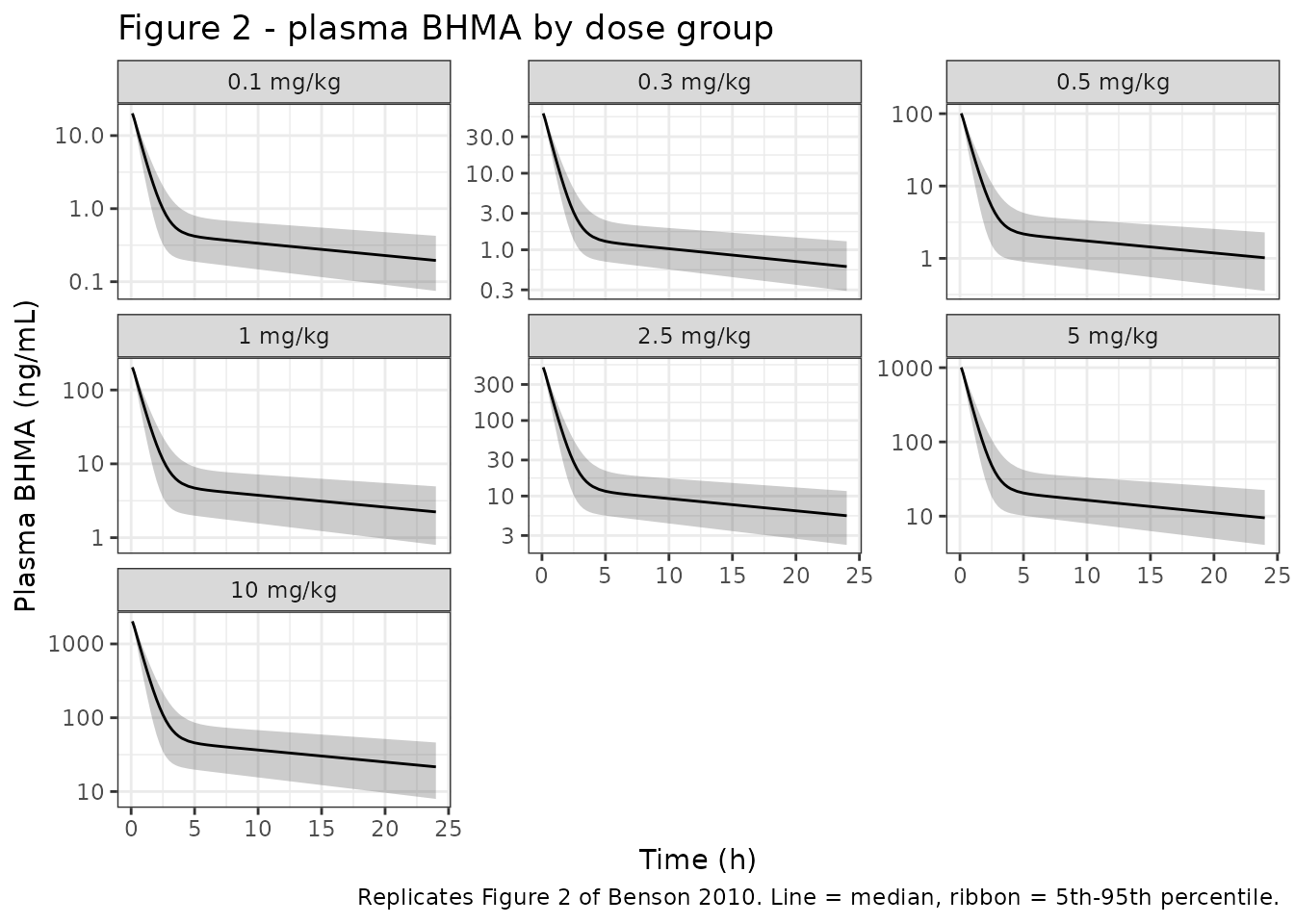
Figure 3A – plasma IFN-alpha by dose group
Benson 2010 Figure 3A plots observed plasma IFN-alpha with the typical predictions from equation 1. The paper’s narrative for this figure is that the rise is “rapid and dose-dependent”, the concentration peaks “at approximately 1 to 2 h”, and it then decreases “rapidly back to zero”.
# Replicates Figure 3A of Benson 2010: plasma IFN-alpha vs. time by dose group.
pd_ribbon <- sim_pd |>
  group_by(treatment, time) |>
  summarise(
    Q05 = quantile(ifna, 0.05), Q50 = quantile(ifna, 0.50),
    Q95 = quantile(ifna, 0.95), .groups = "drop"
  )

ggplot(pd_ribbon, aes(time, Q50)) +
  geom_ribbon(aes(ymin = Q05, ymax = Q95), alpha = 0.25) +
  geom_line() +
  facet_wrap(~treatment) +
  coord_cartesian(xlim = c(0, 12)) +
  labs(
    x = "Time (h)", y = "Plasma IFN-alpha (IU/mL)",
    title = "Figure 3A - plasma IFN-alpha by dose group",
    caption = "Replicates Figure 3A of Benson 2010. Line = median, ribbon = 5th-95th percentile."
  ) +
  theme_bw()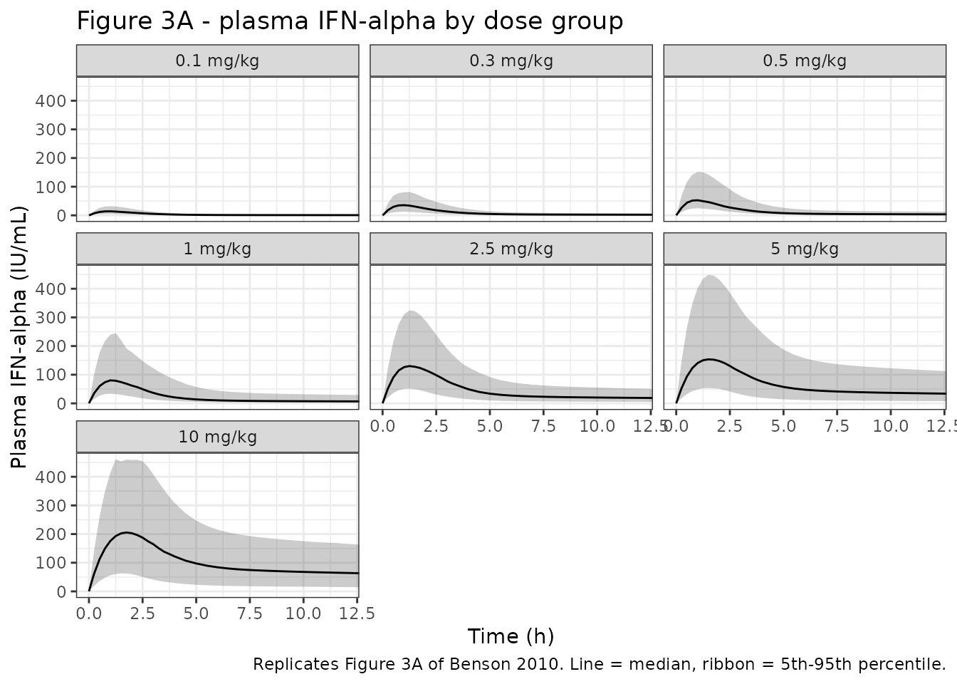
Figure 1 – the saturating concentration-response
Figure 1 of the paper is the schematic: plasma BHMA drives IFN-alpha synthesis through a saturating Emax function. The consequence the authors tested – and the reason the Emax model beat a linear drug effect by dAIC = -22.9 – is that the IFN-alpha response saturates while exposure does not.
typ_peaks <- sim_typ |>
  group_by(treatment, dose_mgkg) |>
  summarise(
    cmax   = max(Cc),
    tmax   = time[which.max(Cc)],
    ifmax  = max(ifna),
    iftmax = time[which.max(ifna)],
    .groups = "drop"
  ) |>
  arrange(dose_mgkg) |>
  mutate(
    cmax_rel  = cmax / cmax[1],
    ifmax_rel = ifmax / ifmax[1]
  )

typ_peaks |>
  select(treatment, cmax, cmax_rel, ifmax, ifmax_rel, iftmax) |>
  rename(
    "Dose"                      = treatment,
    "Cmax (ng/mL)"              = cmax,
    "Cmax relative to 0.1 mg/kg" = cmax_rel,
    "Peak IFN-alpha (IU/mL)"    = ifmax,
    "Peak IFN relative to 0.1 mg/kg" = ifmax_rel,
    "Time of IFN peak (h)"      = iftmax
  ) |>
  knitr::kable(
    digits = c(0, 1, 1, 1, 2, 2),
    caption = paste(
      "Typical-value exposure and IFN-alpha response across the dose range.",
      "Exposure is exactly dose-proportional (linear PK); the IFN-alpha",
      "response is strongly sub-proportional, which is the saturation the",
      "Emax model of equation 1 encodes."
    )
)| Dose | Cmax (ng/mL) | Cmax relative to 0.1 mg/kg | Peak IFN-alpha (IU/mL) | Peak IFN relative to 0.1 mg/kg | Time of IFN peak (h) |
|---|---|---|---|---|---|
| 0.1 mg/kg | 20.2 | 1 | 14.3 | 1.00 | 0.92 |
| 0.3 mg/kg | 60.6 | 3 | 36.6 | 2.56 | 0.98 |
| 0.5 mg/kg | 101.1 | 5 | 53.5 | 3.75 | 1.03 |
| 1 mg/kg | 202.2 | 10 | 83.0 | 5.81 | 1.12 |
| 2.5 mg/kg | 505.4 | 25 | 128.5 | 9.00 | 1.31 |
| 5 mg/kg | 1010.8 | 50 | 162.6 | 11.39 | 1.51 |
| 10 mg/kg | 2021.6 | 100 | 193.2 | 13.54 | 1.74 |
# Structural gate for the paper's central model-selection conclusion (Emax
# beats linear, dAIC = -22.9). Deterministic: this runs on the typical-value
# solve, so both sides use the same parameters and a tight bound is correct.
dose_ratio  <- max(typ_peaks$dose_mgkg) / min(typ_peaks$dose_mgkg)  # 100-fold
cmax_ratio  <- typ_peaks$cmax_rel[nrow(typ_peaks)]
ifmax_ratio <- typ_peaks$ifmax_rel[nrow(typ_peaks)]

stopifnot(
  # Linear PK: a 100-fold dose gives a 100-fold Cmax, to numerical accuracy.
  abs(cmax_ratio / dose_ratio - 1) < 0.01,
  # Saturating PD: the same 100-fold dose gives well under a 20-fold response.
  ifmax_ratio < 20,
  # ... and the response still increases substantially with dose, so the
  # saturation is not a degenerate flat line.
  ifmax_ratio > 5
)
c(dose_ratio = dose_ratio, cmax_ratio = cmax_ratio, ifmax_ratio = ifmax_ratio)
#>  dose_ratio  cmax_ratio ifmax_ratio
#>    100.0000    100.0000     13.5377
PKNCA validation
NCA is run on the stochastic PK cohort (the three PK-only dose groups), with the dose group as the treatment grouping variable so results can be compared per arm.
sim_nca <- sim_pk |>
  dplyr::filter(!is.na(Cc)) |>
  # Per subject, keep Cc >= 1e-6 * Cmax after the peak: below that the ODE integrator has no relative accuracy left.
  dplyr::group_by(id) |>
  dplyr::filter(time <= time[which.max(Cc)] | Cc >= 1e-6 * max(Cc)) |>
  dplyr::ungroup() |>
  dplyr::select(id, time, Cc, treatment)

# Guarantee a time = 0 row per (id, treatment). For an extravascular dose the
# pre-dose concentration is 0, which is the value PKNCA needs to anchor AUC.
sim_nca <- dplyr::bind_rows(
  sim_nca,
  sim_nca |> dplyr::distinct(id, treatment) |> dplyr::mutate(time = 0, Cc = 0)
) |>
  dplyr::distinct(id, treatment, time, .keep_all = TRUE) |>
  dplyr::arrange(id, treatment, time)

conc_obj <- PKNCA::PKNCAconc(sim_nca, Cc ~ time | treatment + id)

dose_df <- events_pk |>
  dplyr::filter(evid == 1) |>
  dplyr::select(id, time, amt, treatment) |>
  dplyr::mutate(treatment = factor(treatment, levels = sprintf("%g mg/kg", pk_doses)))

dose_obj <- PKNCA::PKNCAdose(dose_df, amt ~ time | treatment + id)

intervals <- data.frame(
  start = 0, end = Inf,
  cmax = TRUE, tmax = TRUE, aucinf.obs = TRUE, half.life = TRUE
)

nca_res <- PKNCA::pk.nca(PKNCA::PKNCAdata(conc_obj, dose_obj, intervals = intervals))

nca_tab <- as.data.frame(nca_res) |>
  dplyr::filter(PPTESTCD %in% c("cmax", "tmax", "aucinf.obs", "half.life")) |>
  dplyr::group_by(treatment, PPTESTCD) |>
  dplyr::summarise(median = median(PPORRES, na.rm = TRUE), .groups = "drop") |>
  tidyr::pivot_wider(names_from = PPTESTCD, values_from = median)

nca_tab |>
  dplyr::rename(
    "Dose"                    = treatment,
    "Cmax (ng/mL)"            = cmax,
    "Tmax (h)"                = tmax,
    "AUC0-inf (ng*h/mL)"      = aucinf.obs,
    "t1/2 (h)"                = half.life
  ) |>
  knitr::kable(
    digits = 2,
    caption = "Median simulated NCA parameters for plasma BHMA, by dose group."
)| Dose | AUC0-inf (ng*h/mL) | Cmax (ng/mL) | t1/2 (h) | Tmax (h) |
|---|---|---|---|---|
| 0.1 mg/kg | 29.60 | 20.24 | 18.46 | 0.1 |
| 1 mg/kg | 309.76 | 202.95 | 18.86 | 0.1 |
| 5 mg/kg | 1443.94 | 1010.70 | 18.25 | 0.1 |
Comparison against published quantities
Benson 2010 publishes no NCA table, so there is nothing to feed
nlmixr2lib::ncaComparisonTable(). What the paper does
publish is a set of derived quantities scattered through the Results and
Discussion, each of which is an independent consequence of the tabulated
parameters. Reproducing them is the substantive check, and each is
deterministic – computed either from the ini() values
themselves or from the typical-value solve – so a tight tolerance is the
correct gate here.
ui  <- rxode2::rxode(mod)
fix <- setNames(ui$theta, names(ui$theta))
smax_hat <- exp(fix[["lsmax"]])
ec50_hat <- exp(fix[["lec50"]])
kout_hat <- exp(fix[["lkout"]])
cl_hat   <- exp(fix[["lcl"]])
vc_hat   <- exp(fix[["lvc"]])
vp_hat   <- exp(fix[["lvp"]])
q_hat    <- exp(fix[["lq"]])

# 1. Maximum attainable IFN-alpha response = Smax / kout.
max_response <- smax_hat / kout_hat

# 2. IFN-alpha half-life. Measured on a DECAY-ONLY solve: a bolus into the
#    ifna state with no BHMA dose leaves Cc = 0, so production is zero and the
#    pool decays at exactly kout. Measuring the tail of the coupled solve
#    instead would read the PK washout, not kout (the drug keeps producing).
decay_times <- seq(0.05, 6, by = 0.05)     # post-bolus only; nothing to drop later
decay_ev <- bind_rows(
  tibble(id = 1:2, time = 0, amt = 100, evid = 1L,
         cmt = "ifna", dvid = NA_integer_),
  tidyr::crossing(id = 1:2, time = decay_times) |>
    mutate(amt = NA_real_, evid = 0L, cmt = NA_character_, dvid = 2L)
) |>
  arrange(id, time, desc(evid))

decay <- rxode2::rxSolve(mod_typ, events = decay_ev, useLinCmt = FALSE) |>
  as.data.frame() |>
  dplyr::filter(id == 1)
#> ℹ omega/sigma items treated as zero: 'etalcl', 'etalsmax'
#> Warning: multi-subject simulation without without 'omega'
stopifnot(all(decay$Cc == 0))                       # no drug -> no production
kout_obs <- -unname(coef(lm(log(ifna) ~ time, data = decay))[2])
ifn_halflife_min <- 60 * log(2) / kout_obs

# 3. Apparent clearance recovered from the typical-value NCA. Dose / AUCinf on
#    a zeroRe solve must return CL/F exactly, so this is a pure numerical check.
auc_typ <- sim_typ |>
  group_by(dose_mgkg) |>
  summarise(
    auc  = sum(diff(time) * (head(Cc, -1) + tail(Cc, -1)) / 2),
    ctail = Cc[which.max(time)],
    # Keep Cc >= 1e-6 * Cmax: below that the ODE integrator has no relative accuracy left.
    lz    = {
      ok <- Cc >= 1e-6 * max(Cc)
      -unname(coef(lm(log(tail(Cc[ok], 40)) ~ tail(time[ok], 40)))[2])
    },
    .groups = "drop"
  ) |>
  mutate(
    aucinf = auc + ctail / lz,
    clf    = dose_mgkg * 1e6 / aucinf / 1000,   # mg/kg / (ng*h/mL) -> L/h/kg
    thalf  = log(2) / lz
  )

# 4. Closed-form terminal half-life of the two-compartment disposition.
kel <- cl_hat / vc_hat; k12 <- q_hat / vc_hat; k21 <- q_hat / vp_hat
ssum <- kel + k12 + k21
beta <- 0.5 * (ssum - sqrt(ssum^2 - 4 * kel * k21))
thalf_closed <- log(2) / beta

claims <- tibble::tribble(
  ~Quantity, ~`Benson 2010 states`, ~Model,
  "Maximum attainable IFN-alpha response, Smax/kout (IU/mL)",
    "306 (Discussion)",              round(max_response, 1),
  "IFN-alpha half-life (min)",
    "ca. 43 (Discussion)",           round(ifn_halflife_min, 1),
  "IFN-alpha half-life (h)",
    "ca. 0.7 (Discussion)",          round(ifn_halflife_min / 60, 2),
  "Apparent clearance CL/F (L/h/kg)",
    "3.45 (Table 1)",                round(mean(auc_typ$clf), 3),
  "Apparent peripheral volume V3/F (L/kg)",
    "ca. 40 (Discussion)",           round(vp_hat, 1),
  "Time of maximum plasma BHMA (h)",
    "within 0.1 (Results)",          max(typ_peaks$tmax),
  "Terminal PK half-life (h)",
    "not stated; closed form",       round(thalf_closed, 2)
)

knitr::kable(
  claims,
  caption = "Published derived quantities reproduced from the packaged model."
)| Quantity | Benson 2010 states | Model |
|---|---|---|
| Maximum attainable IFN-alpha response, Smax/kout (IU/mL) | 306 (Discussion) | 306.900 |
| IFN-alpha half-life (min) | ca. 43 (Discussion) | 43.400 |
| IFN-alpha half-life (h) | ca. 0.7 (Discussion) | 0.720 |
| Apparent clearance CL/F (L/h/kg) | 3.45 (Table 1) | 3.451 |
| Apparent peripheral volume V3/F (L/kg) | ca. 40 (Discussion) | 39.700 |
| Time of maximum plasma BHMA (h) | within 0.1 (Results) | 0.100 |
| Terminal PK half-life (h) | not stated; closed form | 18.270 |
stopifnot(
  # Smax / kout -- the paper prints 306; 294 / 0.958 = 306.89, so the residual
  # is the paper's own rounding of kout to 0.96.
  abs(max_response - 306) < 2,
  # kout recovered from the decay-only solve must return the ini() value to
  # solver accuracy, and hence the paper's "ca. 43 min".
  abs(kout_obs - kout_hat) < 1e-4,
  abs(ifn_halflife_min - 43) < 1.5,
  # Dose / AUCinf on the typical-value solve must return CL/F. Both sides use
  # the same parameters, so the only error is trapezoidal, and it is < 0.1%.
  all(abs(auc_typ$clf / cl_hat - 1) < 0.01),
  # Linear PK: CL/F is identical across the seven dose levels.
  diff(range(auc_typ$clf)) / mean(auc_typ$clf) < 1e-3,
  # Terminal half-life from the solve matches the two-compartment closed form.
  all(abs(auc_typ$thalf - thalf_closed) < 0.1),
  # Tmax at every dose is at or before the paper's stated 0.1 h; the typical
  # grid resolves 0.01 h, so this is a real bound, not a grid artefact.
  all(typ_peaks$tmax <= 0.11),
  # The typical-value IFN-alpha peak at the top dose is the single quantity
  # that depends on ALL of Smax, SC50, kout and the PK at once, so pinning it
  # tightly is the strongest available check on SC50 (which none of the gates
  # above constrain). It is fully deterministic -- a zeroRe solve on a fixed
  # grid, no RNG anywhere -- so a 1 IU/mL band is correct rather than
  # optimistic. Measured sensitivity of this number: halving or doubling SC50
  # moves it 14-16%, Smax 50-100%, kout 40-51%, CL 11-16%, Vc 5-13%.
  abs(typ_peaks$ifmax[typ_peaks$dose_mgkg == 10] - 193.2) < 1.0
)
Cohort-level checks
Two claims in the paper are properties of the simulated cohort rather than of the typical individual, so they are gated on the median and on robust quantiles, never on the extreme of a random draw (an extreme is not reproducible across rxode2 builds or solver-thread counts).
cohort_peaks <- sim_pd |>
  group_by(treatment, dose_mgkg, id) |>
  summarise(
    ifmax   = max(ifna),
    iftmax  = time[which.max(ifna)],
    smax_i  = first(smax),          # this animal's own Smax, after its eta
    kout_i  = first(kout),
    .groups = "drop"
  )

peak_summary <- cohort_peaks |>
  group_by(treatment, dose_mgkg) |>
  summarise(
    `Median peak IFN (IU/mL)` = median(ifmax),
    `90th pct peak (IU/mL)`   = quantile(ifmax, 0.9),
    `Median time of peak (h)` = median(iftmax),
    .groups = "drop"
  ) |>
  arrange(dose_mgkg) |>
  select(-dose_mgkg) |>
  rename("Dose" = treatment)

knitr::kable(
  peak_summary, digits = 1,
  caption = paste(
    "Simulated per-animal IFN-alpha peaks. Benson 2010 Results describe the",
    "observed peak as occurring 'at approximately 1 to 2 h around 300 IU/ml'."
  )
)| Dose | Median peak IFN (IU/mL) | 90th pct peak (IU/mL) | Median time of peak (h) |
|---|---|---|---|
| 0.1 mg/kg | 14.1 | 28.8 | 1.0 |
| 0.3 mg/kg | 35.7 | 71.7 | 1.0 |
| 0.5 mg/kg | 52.8 | 109.0 | 1.0 |
| 1 mg/kg | 80.6 | 178.5 | 1.2 |
| 2.5 mg/kg | 131.2 | 268.0 | 1.2 |
| 5 mg/kg | 154.0 | 390.2 | 1.5 |
| 10 mg/kg | 205.4 | 426.1 | 1.8 |
top      <- cohort_peaks |> filter(dose_mgkg == max(dose_mgkg))
typ_peak <- typ_peaks$ifmax[typ_peaks$dose_mgkg == max(typ_peaks$dose_mgkg)]

stopifnot(
  # Timing: the paper says the peak is at approximately 1 to 2 h. The median
  # over the cohort is the reproducible statistic; the window is widened by
  # half an hour on each side so that it is not a race against the draw.
  median(top$iftmax) > 0.5, median(top$iftmax) < 2.5,
  # Magnitude: the IFN-alpha ODE is linear in Smax, so each animal's peak is
  # exactly proportional to its own Smax and the COHORT MEDIAN is an unbiased
  # estimate of the typical-value peak. It is still a sample median of a
  # lognormal with omega = 0.63, so it carries real sampling noise: over 40 R
  # seeds at n = 100 per arm the ratio to the typical value ranged
  # [0.826, 1.197] with sd 0.100 and mean 0.987. The 45% band is ~4.5 sd and
  # more than twice the worst observed excursion, yet still bites -- halving
  # or doubling Smax moves this by 50-100%, kout by 40-51%, and the tight
  # deterministic gate above already pins the typical value to +/- 1 IU/mL.
  abs(median(top$ifmax) / typ_peak - 1) < 0.45,
  # No animal can exceed its OWN structural ceiling Smax_i / kout_i. Computed
  # from each animal's simulated parameters rather than from a quantile of the
  # eta distribution, so it is an exact invariant of the model rather than a
  # bound that a large enough cohort would eventually breach by chance.
  all(top$ifmax <= top$smax_i / top$kout_i)
)
The paper’s “around 300 IU/ml” is the observed peak
in the highest dose groups, not the typical-value prediction, and the
two should not be expected to coincide. Because the IFN-alpha ODE is
linear in Smax, each animal’s peak is exactly proportional
to its own Smax, so the 70% CV on Smax carries
straight through to the distribution of peaks: at 10 mg/kg the typical
animal peaks near 193 IU/mL against a structural ceiling
Smax/kout of 307 IU/mL, while the upper part of the cohort
reaches 300 IU/mL and beyond (each animal’s ceiling scales with its own
Smax, so individual peaks are not bounded by the typical
animal’s 307). All three readings – the typical peak, the ceiling, and
the observed peak the paper quotes – are consistent consequences of the
same parameters. The gate above is therefore placed on the cohort
median, which estimates a reproducible quantity, and never on which tail
a particular draw happens to produce.
ggplot(top, aes(ifmax)) +
  geom_histogram(bins = 25, fill = "grey70", colour = "white") +
  geom_vline(xintercept = median(top$ifmax), linetype = "dashed") +
  geom_vline(xintercept = 300, colour = "firebrick") +
  labs(
    x = "Per-animal peak plasma IFN-alpha (IU/mL)", y = "Animals",
    title = "Distribution of peak IFN-alpha at 10 mg/kg",
    caption = paste(
      "Dashed = cohort median; red = the 'around 300 IU/ml' the paper reports",
      "for the observed peak in the highest dose groups."
    )
  ) +
  theme_bw()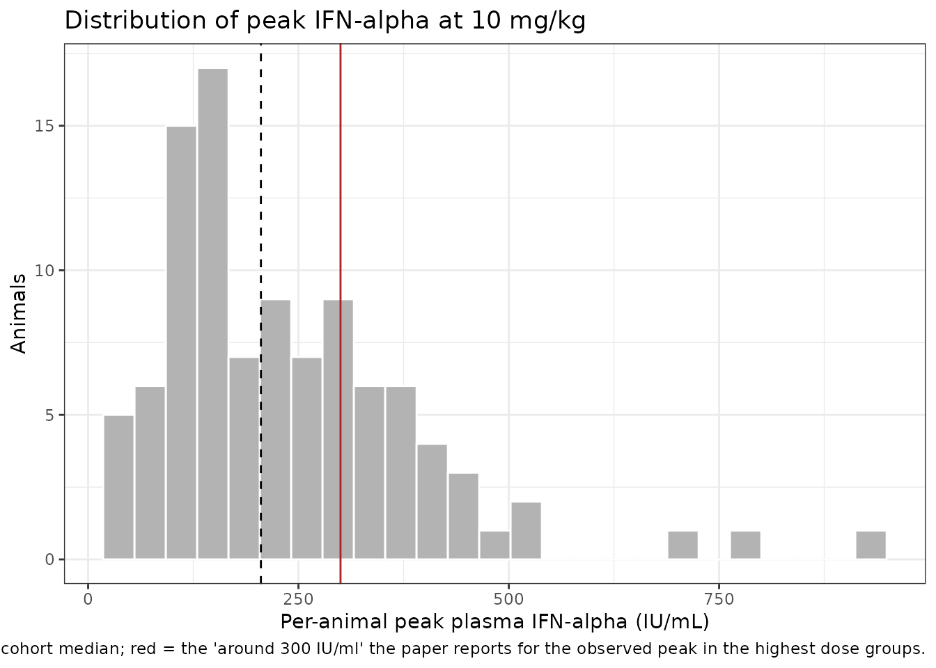
Assumptions and deviations
All PK parameters are apparent (
/F). Benson 2010 had no intravenous arm, so bioavailability could not be estimated; the Discussion states that “the volume of distribution (V) of ca. 40 liters/kg must be regarded as the V/F ratio” and speculates that F may be as low as ca. 5% given BHMA’s low solubility (ca. 6 ug/mL). The model file recordsCL,V2,QandV3at their published values and names them apparent in everylabel(); no bioavailability term is introduced, because the paper estimates none.Doses must be supplied in mg/kg. Every disposition parameter is reported per kilogram body weight, so the compartment amounts are in mg/kg and
Cc = 1000 * central / vcis in ng/mL. Body weight is therefore not a covariate of this model; supplying an absolute mg dose would misstate every concentration by the animal’s weight.IIV variances are back-transformed from the published CVs. Table 1 and Table 2 report “IIV of CL (%)” = 38 and “IIV of Smax (%)” = 70. The Methods state that the IIV “is expressed as the percent CV” and equation 3 is the lognormal
Pi = theta * exp(eta_i), soomega^2 = log(CV^2 + 1)was used rather than taking the percentage asomegadirectly. The difference is small for CL (0.1349 vs 0.1444) and material for Smax (0.3988 vs 0.4900).No Hill exponent. Equation 1 is written as an ordinary Emax function and Table 2 lists no gamma; the Results describe the winning model as “the ordinary Emax model”, and the Table 2 footnote says only “an indirect response model (equation 1)”. Two places use the word “sigmoid” – the Methods (“a sigmoid saturating concentration-response relationship”) and the Figure 1 legend (“a sigmoid Emax function”) – but neither is accompanied by an estimated exponent anywhere in the paper, and equation 1 as printed has none. Read as the customary description of the shape of a saturating concentration-response curve; no exponent was introduced.
The IFN-alpha baseline is a structural zero, not an estimated parameter. Basal IFN-alpha was below the 0.3 IU/mL assay LOQ in every animal, so the paper fixed it at zero. The model encodes
ifna(0) <- 0and a production term with nokinoffset. A consequence worth knowing before reusing this model: with the baseline at zero there is no turnover in the absence of drug, so the model cannot describe a pre-dose or placebo IFN-alpha profile.Residual-error models are assigned by the units of the tabulated estimate. Benson 2010 presents both an additive (equation 4) and a proportional (equation 5) residual model in the Methods but does not say in prose which stage used which. Table 1 reports the PK residual error as “46 (%)” and Table 2 reports the PD residual error as “65 (IU/ml)”; the units identify the proportional model for the PK and the additive model for the PD. This is an inference from the tables, not an explicit statement in the text.
Non-reproducible arithmetic in the Discussion’s unbound potency. The Discussion converts the total
SC50of 135 ng/mL to an unbound potency of “ca. 125 nM” using the mouse plasma free fraction of 0.33. Recomputing with the molecular weight of BHMA (C15H17N5O3, 315.3 g/mol) gives135 * 0.33 / 315.3= 141 nM, about 13% higher; the paper’s 125 nM back-solves to a molecular weight of ca. 356 g/mol or a free fraction of ca. 0.29. The discrepancy is confined to that one derived sentence – it is not used anywhere in the fitted model – and the packagedlec50is the tabulated total plasmaSC50of 135 ng/mL, exactly as estimated. The ca. fourfold gap the paper draws between its in vivo unboundSC50and the ca. 30 nM human replicon potency is unaffected in direction or order of magnitude.Sequential fit, replicated as a single model file. The paper fitted the PK first and then fixed the PK parameters at their typical population values while fitting the PD, using individual PK parameters only for the animals that had them. The packaged file carries both stages in one model, which is the form a downstream user simulates from; refitting it as a joint model would not reproduce the published estimates.
Composite sampling is not reproduced. The paper used a matrix design in which each animal contributes only a few samples. The virtual cohorts above sample every animal densely, which is appropriate for validating the structural model but does not reproduce the information content of the original design.
Assay limits of quantification are not applied. Simulated concentrations are reported without censoring at the 0.5 ng/mL (BHMA) and 0.3 IU/mL (IFN-alpha) limits, so late-time BHMA values in the figures fall below what the study could have measured.