Piperacillin + tazobactam in infants (Cohen-Wolkowiez 2014)
Source:vignettes/articles/CohenWolkowiez_2014_piperacillin_tazobactam.Rmd
CohenWolkowiez_2014_piperacillin_tazobactam.RmdModel and source
Cohen-Wolkowiez et al. 2014 developed independent one-compartment
population PK models for piperacillin and tazobactam (coadministered as
the 8:1 fixed-ratio combination piperacillin-tazobactam) in 32
critically ill premature and term infants under 61 days postnatal age
(PNA). Both drugs share the same study population, the same dosing
regimen, and the same plasma sampling scheme; the two structural models
differ in their covariate composition on clearance. This vignette walks
the paper’s narrative for both drugs and uses each
modellib() entry at the point in the narrative where the
corresponding model is introduced.
- Citation (piperacillin): Cohen-Wolkowiez M, Watt KM, Zhou C, Bloom BT, Poindexter B, Castro L, Gao J, Capparelli EV, Benjamin DK Jr, Smith PB. Developmental pharmacokinetics of piperacillin and tazobactam using plasma and dried blood spots from infants. Antimicrob Agents Chemother. 2014;58(5):2856-2865. doi:10.1128/AAC.02139-13.
- Citation (tazobactam): Cohen-Wolkowiez M, Watt KM, Zhou C, Bloom BT, Poindexter B, Castro L, Gao J, Capparelli EV, Benjamin DK Jr, Smith PB. Developmental pharmacokinetics of piperacillin and tazobactam using plasma and dried blood spots from infants. Antimicrob Agents Chemother. 2014;58(5):2856-2865. doi:10.1128/AAC.02139-13.
- Article: https://doi.org/10.1128/AAC.02139-13
Population
Thirty-two infants were enrolled 2010-2011 at four US neonatal intensive care units in an open-label, prospective, early-phase PK and safety study of intravenous piperacillin-tazobactam in young infants under 61 days postnatal age with suspected systemic infection. Enrollment was stratified by gestational age (GA) at birth and postnatal age (PNA) into four cohorts: cohort 1 (n = 12, GA < 32 wk, PNA < 14 d), cohort 2 (n = 9, GA < 32 wk, PNA >= 14 d), cohort 3 (n = 8, GA >= 32 wk, PNA < 14 d), and cohort 4 (n = 3, GA >= 32 wk, PNA >= 14 d). Cohorts 1-3 received piperacillin 80 mg/kg every 8 h IV (30-min infusion); cohort 4 received 100 mg/kg every 8 h. Demographics across the pooled cohort (Cohen-Wolkowiez 2014 Table 1): median GA 30 weeks (range 23-40), median PNA 8 days (1-60), median postmenstrual age (PMA) 32 weeks (25-48), median weight 1.439 kg (0.473-3.990), median serum creatinine 0.8 mg/dL (0.3-2.0). 63% of infants received concurrent gentamicin, 13% dopamine, 6% epinephrine; 63% were male. 128 timed plasma piperacillin and tazobactam samples (median 4 samples per infant) were retained for the population PK analysis. Concurrent dried-blood-spot samples were also collected; the structural PK models extracted here were fit to plasma alone.
The same metadata is available programmatically via
readModelDb("CohenWolkowiez_2014_piperacillin")()$population
(and the equivalent for tazobactam).
Source trace
The per-parameter origin is recorded inline next to each
ini() entry in
inst/modeldb/specificDrugs/CohenWolkowiez_2014_piperacillin.R
and
inst/modeldb/specificDrugs/CohenWolkowiez_2014_tazobactam.R.
The table below collects them in one place for review.
Piperacillin (Cohen-Wolkowiez 2014 Table 3 final PMA-based model)
| Equation / parameter | Value | Source location |
|---|---|---|
lcl (typical CL per kg body weight, L/kg/h, at PMA = 33
wk) |
log(0.080) |
Table 3: typical CL value 0.080 L/kg/h (RSE 7.9%) |
lvc (typical V per kg body weight, L/kg) |
log(0.42) |
Table 3: typical V value 0.42 L/kg (RSE 9.6%) |
e_wt_cl (linear WT exponent on CL, unitless) |
fixed(1.0) |
Population PK model building paragraph: WT exponent fixed at 1; free body-size and 3/4-power scaling explored and rejected |
e_wt_vc (linear WT exponent on V, unitless) |
fixed(1.0) |
Population PK model building paragraph: WT exponent fixed at 1 |
e_page_cl (power exponent on (PMA / 33 wk) for CL) |
1.76 |
Table 3: PMA covariate 1.76 (RSE 33.6%) |
etalcl (omega_CL on internal scale) |
0.12839 (37% CV) |
Table 3: CL interindividual variability 37% CV (RSE 27.5%); omega^2 = log(1 + CV^2) |
(no etalvc) |
n/a | Population PK model building paragraph: between-subject variability on V fixed to 0 (boundary value) |
propSd (proportional residual error) |
0.33 |
Table 3: proportional residual error 33% CV (RSE 9.9%) |
addSd (additive residual error, mg/L) |
6.90 |
Table 3: plasma additive residual error 6.90 mg/L (RSE 42.6%) |
d/dt(central) (one-compartment IV PK) |
n/a | Population PK model building paragraph: one-compartment structural model selected |
Piperacillin CL covariate equation
CL = theta_CL * WT * (PMA / 33)^COVPMA
|
n/a | Table 2 final piperacillin model row and Population PK model building paragraph |
Tazobactam (Cohen-Wolkowiez 2014 Table 4 final model)
| Equation / parameter | Value | Source location |
|---|---|---|
lcl (typical CL per kg body weight, L/kg/h, at PMA = 33
wk, SCR = 0.5 mg/dL, no concurrent gentamicin) |
log(0.088) |
Table 4: typical CL value 0.088 L/kg/h (RSE 8.9%) |
lvc (typical V per kg body weight, L/kg) |
log(0.57) |
Table 4: typical V value 0.57 L/kg (RSE 5.4%) |
e_wt_cl (linear WT exponent on CL, unitless) |
fixed(1.0) |
Population PK model building paragraph: WT exponent fixed at 1 |
e_wt_vc (linear WT exponent on V, unitless) |
fixed(1.0) |
Population PK model building paragraph: WT exponent fixed at 1 |
e_page_cl (power exponent on (PMA / 33 wk) for CL) |
1.35 |
Table 4: PMA covariate 1.35 (RSE 27.3%) |
e_creat_cl (power exponent on (CREAT / 0.5 mg/dL) for
CL) |
-0.35 |
Table 4: SCR covariate -0.35 (RSE 37.0%) |
e_conmed_gen_cl (multiplicative factor on CL for GENT =
1) |
1.52 |
Table 4: GENT covariate 1.52 (RSE 10.1%) |
etalcl (omega_CL on internal scale) |
0.05154 (23% CV) |
Table 4: CL interindividual variability 23% CV (RSE 34.0%); omega^2 = log(1 + CV^2) |
(no etalvc) |
n/a | Population PK model building paragraph: between-subject variability on V fixed to 0 (boundary value) |
propSd (proportional residual error) |
0.24 |
Table 4: proportional residual error 24% CV (RSE 19.8%) |
addSd (additive residual error, mg/L) |
1.43 |
Table 4: plasma additive residual error 1.43 mg/L (RSE 51.2%) |
d/dt(central) (one-compartment IV PK) |
n/a | Population PK model building paragraph: one-compartment structural model selected |
Tazobactam CL covariate equation
CL = theta_CL * WT * (PMA / 33)^COVPMA * (SCR / 0.5)^COVSCR * COVGENT^GENT
|
n/a | Table 2 final tazobactam model row and Population PK model building paragraph |
Virtual cohort
Original observed concentrations are not publicly available. The simulations below use a virtual cohort whose PMA / WT / SCR distributions mirror the Cohen-Wolkowiez 2014 Table 1 demographics and whose dosing follows the per- cohort protocol assignments (80 mg/kg q8h piperacillin for cohorts 1-3; 100 mg/kg q8h for cohort 4). The tazobactam component is dosed at one-eighth the piperacillin dose (fixed 8:1 piperacillin:tazobactam ratio).
set.seed(2026)

T_INF         <- 0.5   # hour; 30-min IV infusion
DOSE_INTERVAL <- 8     # hours
N_DOSES       <- 5     # five doses to approach steady state

# Per-cohort typical demographics from Cohen-Wolkowiez 2014 Table 1
# (median values; PMA in weeks, WT in kg, SCR in mg/dL, dose in mg/kg).
cohorts <- tibble::tribble(
  ~cohort,            ~n,  ~PMA_wk, ~WT_kg, ~CREAT, ~CONMED_GEN, ~dose_pip_mg_per_kg,
  "cohort 1",         50,  29,      1.109,  0.8,    0,           80,
  "cohort 2",         50,  33,      1.397,  0.8,    1,           80,
  "cohort 3",         50,  39,      3.248,  0.8,    0,           80,
  "cohort 4",         50,  43,      3.050,  0.6,    0,           100
)

# Helper to build one cohort's event table. id_offset shifts subject IDs so
# bind_rows() across cohorts does not collide on `id` (rxode2 silently merges
# duplicate IDs across cohorts).
make_cohort <- function(spec, id_offset, dose_mg_per_kg, drug,
                        ratio_piperacillin_to_tazobactam = 8L) {
  WT_kg <- spec$WT_kg
  per_dose_mg <- if (drug == "piperacillin") {
    dose_mg_per_kg * WT_kg
  } else {
    dose_mg_per_kg * WT_kg / ratio_piperacillin_to_tazobactam
  }
  rows <- vector("list", spec$n)
  for (k in seq_len(spec$n)) {
    sid <- id_offset + k
    ev <- rxode2::et(
      amt   = per_dose_mg,
      rate  = per_dose_mg / T_INF,
      ii    = DOSE_INTERVAL,
      addl  = N_DOSES - 1L,
      cmt   = "central"
    ) |>
      rxode2::et(seq(0, N_DOSES * DOSE_INTERVAL, by = 0.25))
    df <- as.data.frame(ev)
    df$id         <- sid
    df$cohort     <- spec$cohort
    df$WT         <- WT_kg
    df$PAGE       <- spec$PMA_wk / 4.35   # PMA (wk) -> PAGE canonical (months)
    df$CREAT      <- spec$CREAT
    df$CONMED_GEN <- spec$CONMED_GEN
    rows[[k]] <- df
  }
  dplyr::bind_rows(rows)
}

build_events <- function(drug) {
  offsets <- c(0L, cumsum(head(cohorts$n, -1)))
  parts <- lapply(seq_len(nrow(cohorts)), function(i) {
    make_cohort(
      cohorts[i, ],
      id_offset      = offsets[[i]],
      dose_mg_per_kg = cohorts$dose_pip_mg_per_kg[[i]],
      drug           = drug
    )
  })
  ev <- dplyr::bind_rows(parts)
  stopifnot(!anyDuplicated(unique(ev[, c("id", "time", "evid")])))
  ev
}

events_pip <- build_events("piperacillin")
events_taz <- build_events("tazobactam")

# rxode2::et(..., addl = ) encodes the entire repeated-dose schedule as a
# single event row. For PKNCA we need one row per administered dose, so
# expand the schedule analytically using the known cohort + dose layout.
expand_dose_schedule <- function(events, drug,
                                 ratio_piperacillin_to_tazobactam = 8L) {
  one_per_subj <- events |>
    dplyr::filter(!is.na(amt), amt > 0) |>
    dplyr::distinct(id, cohort, .keep_all = TRUE) |>
    dplyr::select(id, cohort)
  dose_times <- seq(0, by = DOSE_INTERVAL, length.out = N_DOSES)
  per_cohort_dose_pip <- setNames(cohorts$dose_pip_mg_per_kg, cohorts$cohort)
  per_cohort_wt       <- setNames(cohorts$WT_kg,              cohorts$cohort)
  tidyr::expand_grid(one_per_subj, time = dose_times) |>
    dplyr::mutate(
      amt = {
        per_kg <- per_cohort_dose_pip[as.character(cohort)]
        if (drug == "tazobactam") per_kg <- per_kg / ratio_piperacillin_to_tazobactam
        per_kg * per_cohort_wt[as.character(cohort)]
      }
    )
}

doses_pip <- expand_dose_schedule(events_pip, "piperacillin")
doses_taz <- expand_dose_schedule(events_taz, "tazobactam")
Simulation
Piperacillin (one-compartment, PMA-based final model)
mod_pip <- readModelDb("CohenWolkowiez_2014_piperacillin")
sim_pip <- rxode2::rxSolve(mod_pip, events = events_pip,
                           keep = c("cohort", "WT", "PAGE"))
#> ℹ parameter labels from comments will be replaced by 'label()'
sim_pip <- as.data.frame(sim_pip)
Tazobactam (one-compartment with PMA + SCR + GENT covariates)
mod_taz <- readModelDb("CohenWolkowiez_2014_tazobactam")
sim_taz <- rxode2::rxSolve(mod_taz, events = events_taz,
                           keep = c("cohort", "WT", "PAGE", "CREAT", "CONMED_GEN"))
#> ℹ parameter labels from comments will be replaced by 'label()'
sim_taz <- as.data.frame(sim_taz)
Replicate published figures
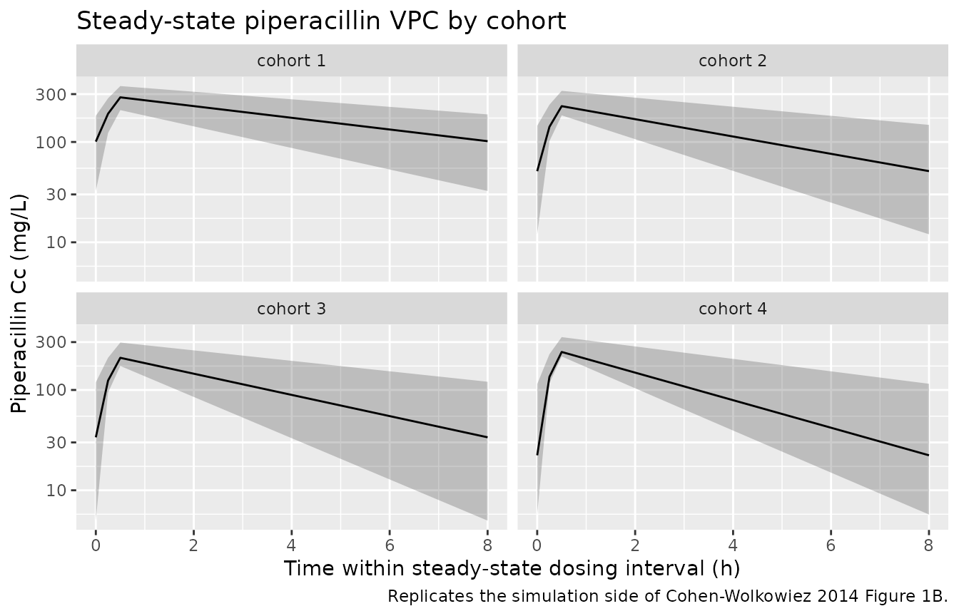
Cohen-Wolkowiez 2014 Figures 1 and 2 are diagnostic plots from the NONMEM fit (observed vs individual predictions, VPC of concentration vs time, CWRES vs population predictions / time). Reproducing the VPC panel against simulated trajectories shows the per-cohort piperacillin and tazobactam profiles across one dosing interval at steady state.
# Reproduces the simulation side of Cohen-Wolkowiez 2014 Figure 1B
# (piperacillin VPC) at steady state: simulated piperacillin
# concentration vs time within the final dosing interval, with 90% prediction
# interval and median by cohort.
ss_window_pip <- sim_pip |>
  dplyr::filter(time >= (N_DOSES - 1) * DOSE_INTERVAL,
                time <= N_DOSES * DOSE_INTERVAL,
                !is.na(Cc)) |>
  dplyr::mutate(time_in_interval = time - (N_DOSES - 1) * DOSE_INTERVAL)

vpc_pip <- ss_window_pip |>
  dplyr::group_by(cohort, time_in_interval) |>
  dplyr::summarise(
    Q05 = quantile(Cc, 0.05, na.rm = TRUE),
    Q50 = quantile(Cc, 0.50, na.rm = TRUE),
    Q95 = quantile(Cc, 0.95, na.rm = TRUE),
    .groups = "drop"
  )

ggplot(vpc_pip, aes(time_in_interval, Q50)) +
  geom_ribbon(aes(ymin = Q05, ymax = Q95), alpha = 0.25) +
  geom_line() +
  facet_wrap(~ cohort) +
  scale_y_log10() +
  labs(
    x = "Time within steady-state dosing interval (h)",
    y = "Piperacillin Cc (mg/L)",
    title = "Steady-state piperacillin VPC by cohort",
    caption = "Replicates the simulation side of Cohen-Wolkowiez 2014 Figure 1B."
  )
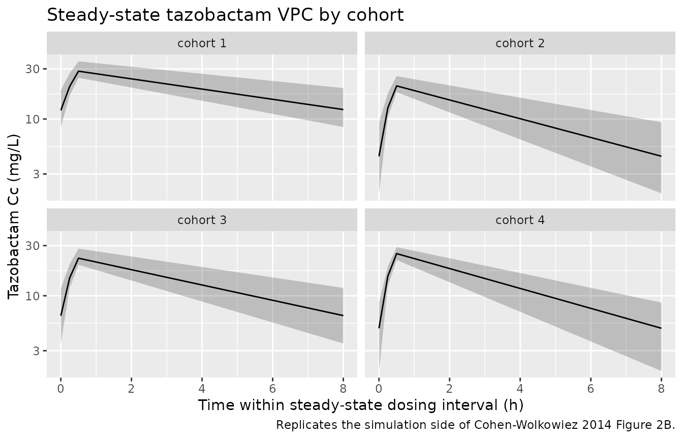
# Reproduces the simulation side of Cohen-Wolkowiez 2014 Figure 2B
# (tazobactam VPC) at steady state.
ss_window_taz <- sim_taz |>
  dplyr::filter(time >= (N_DOSES - 1) * DOSE_INTERVAL,
                time <= N_DOSES * DOSE_INTERVAL,
                !is.na(Cc)) |>
  dplyr::mutate(time_in_interval = time - (N_DOSES - 1) * DOSE_INTERVAL)

vpc_taz <- ss_window_taz |>
  dplyr::group_by(cohort, time_in_interval) |>
  dplyr::summarise(
    Q05 = quantile(Cc, 0.05, na.rm = TRUE),
    Q50 = quantile(Cc, 0.50, na.rm = TRUE),
    Q95 = quantile(Cc, 0.95, na.rm = TRUE),
    .groups = "drop"
  )

ggplot(vpc_taz, aes(time_in_interval, Q50)) +
  geom_ribbon(aes(ymin = Q05, ymax = Q95), alpha = 0.25) +
  geom_line() +
  facet_wrap(~ cohort) +
  scale_y_log10() +
  labs(
    x = "Time within steady-state dosing interval (h)",
    y = "Tazobactam Cc (mg/L)",
    title = "Steady-state tazobactam VPC by cohort",
    caption = "Replicates the simulation side of Cohen-Wolkowiez 2014 Figure 2B."
  )
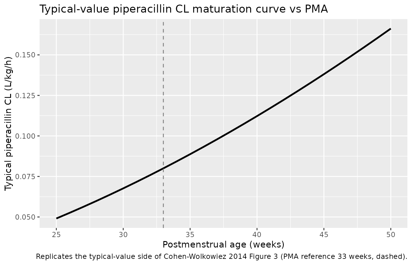
# Reproduces the typical-value side of Cohen-Wolkowiez 2014 Figure 3:
# population-typical piperacillin clearance (per kg) vs PMA. With
# random effects zeroed, the curve shows the PMA maturation only
# (since linear WT scaling has no effect on per-kg CL).
typical_pip <- rxode2::zeroRe(mod_pip)
#> ℹ parameter labels from comments will be replaced by 'label()'
pma_grid <- seq(25, 50, by = 1)
typical_cl <- vapply(pma_grid, function(pma_wk) {
  ev1 <- rxode2::et(amt = 80, rate = 80 / T_INF, cmt = "central") |>
    rxode2::et(c(0.5, 1, 8))
  ev1$WT <- 1
  ev1$PAGE <- pma_wk / 4.35
  out <- rxode2::rxSolve(typical_pip, ev1)
  # CL = -V * ln(C(t2)/C(t1)) / (t2 - t1); use post-infusion samples
  out <- as.data.frame(out)
  post <- out[out$time %in% c(1, 8), ]
  V <- exp(log(0.42))   # vc per kg for the typical model
  cl <- -V * (log(post$Cc[post$time == 8]) - log(post$Cc[post$time == 1])) / (8 - 1)
  cl
}, numeric(1))
#> ℹ omega/sigma items treated as zero: 'etalcl'
#> ℹ omega/sigma items treated as zero: 'etalcl'
#> ℹ omega/sigma items treated as zero: 'etalcl'
#> ℹ omega/sigma items treated as zero: 'etalcl'
#> ℹ omega/sigma items treated as zero: 'etalcl'
#> ℹ omega/sigma items treated as zero: 'etalcl'
#> ℹ omega/sigma items treated as zero: 'etalcl'
#> ℹ omega/sigma items treated as zero: 'etalcl'
#> ℹ omega/sigma items treated as zero: 'etalcl'
#> ℹ omega/sigma items treated as zero: 'etalcl'
#> ℹ omega/sigma items treated as zero: 'etalcl'
#> ℹ omega/sigma items treated as zero: 'etalcl'
#> ℹ omega/sigma items treated as zero: 'etalcl'
#> ℹ omega/sigma items treated as zero: 'etalcl'
#> ℹ omega/sigma items treated as zero: 'etalcl'
#> ℹ omega/sigma items treated as zero: 'etalcl'
#> ℹ omega/sigma items treated as zero: 'etalcl'
#> ℹ omega/sigma items treated as zero: 'etalcl'
#> ℹ omega/sigma items treated as zero: 'etalcl'
#> ℹ omega/sigma items treated as zero: 'etalcl'
#> ℹ omega/sigma items treated as zero: 'etalcl'
#> ℹ omega/sigma items treated as zero: 'etalcl'
#> ℹ omega/sigma items treated as zero: 'etalcl'
#> ℹ omega/sigma items treated as zero: 'etalcl'
#> ℹ omega/sigma items treated as zero: 'etalcl'
#> ℹ omega/sigma items treated as zero: 'etalcl'

df_typical <- tibble::tibble(PMA_wk = pma_grid, CL_per_kg = typical_cl)
ggplot(df_typical, aes(PMA_wk, CL_per_kg)) +
  geom_line(linewidth = 1) +
  geom_vline(xintercept = 33, linetype = "dashed", colour = "grey50") +
  labs(
    x = "Postmenstrual age (weeks)",
    y = "Typical piperacillin CL (L/kg/h)",
    title = "Typical-value piperacillin CL maturation curve vs PMA",
    caption = "Replicates the typical-value side of Cohen-Wolkowiez 2014 Figure 3 (PMA reference 33 weeks, dashed)."
  )
PKNCA validation
Steady-state NCA per cohort. The fixed-effect (typical-value) trajectory is the appropriate target for comparison against the empirical-Bayesian summary the source paper reports in Table 5; full-IIV simulations are also computed to illustrate the spread.
Piperacillin (steady state, AUC0-tau, Cmax,ss, Cmin,ss)
tau <- DOSE_INTERVAL
start_ss <- (N_DOSES - 1) * tau
end_ss   <- N_DOSES * tau

sim_nca_pip <- sim_pip |>
  dplyr::filter(!is.na(Cc), time >= start_ss, time <= end_ss) |>
  dplyr::select(id, time, Cc, cohort)

dose_nca_pip <- doses_pip |>
  dplyr::filter(time >= start_ss, time <= end_ss)

conc_obj_pip <- PKNCA::PKNCAconc(sim_nca_pip, Cc ~ time | cohort + id,
                                 concu = "mg/L", timeu = "hr")
dose_obj_pip <- PKNCA::PKNCAdose(dose_nca_pip, amt ~ time | cohort + id,
                                 doseu = "mg")
intervals_pip <- data.frame(
  start    = start_ss,
  end      = end_ss,
  cmax     = TRUE,
  tmax     = TRUE,
  cmin     = TRUE,
  auclast  = TRUE,
  cav      = TRUE,
  ctrough  = TRUE
)
nca_pip <- PKNCA::pk.nca(PKNCA::PKNCAdata(conc_obj_pip, dose_obj_pip,
                                          intervals = intervals_pip))
knitr::kable(summary(nca_pip),
caption = "Simulated steady-state piperacillin NCA by cohort.")| Interval Start | Interval End | cohort | N | AUClast (hr*mg/L) | Cmax (mg/L) | Cmin (mg/L) | Tmax (hr) | Cav (mg/L) | Ctrough (mg/L) |
|---|---|---|---|---|---|---|---|---|---|
| 32 | 40 | cohort 1 | 50 | 1340 [33.7] | 275 [17.9] | 88.7 [61.0] | 0.500 [0.500, 0.500] | 167 [33.7] | NC |
| 32 | 40 | cohort 2 | 50 | 991 [40.5] | 237 [18.1] | 50.0 [95.3] | 0.500 [0.500, 0.500] | 124 [40.5] | NC |
| 32 | 40 | cohort 3 | 50 | 775 [45.2] | 214 [17.5] | 28.4 [150] | 0.500 [0.500, 0.500] | 96.8 [45.2] | NC |
| 32 | 40 | cohort 4 | 50 | 789 [34.6] | 247 [12.6] | 22.9 [99.7] | 0.500 [0.500, 0.500] | 98.6 [34.6] | NC |
Tazobactam (steady state, AUC0-tau, Cmax,ss, Cmin,ss)
sim_nca_taz <- sim_taz |>
  dplyr::filter(!is.na(Cc), time >= start_ss, time <= end_ss) |>
  dplyr::select(id, time, Cc, cohort)

dose_nca_taz <- doses_taz |>
  dplyr::filter(time >= start_ss, time <= end_ss)

conc_obj_taz <- PKNCA::PKNCAconc(sim_nca_taz, Cc ~ time | cohort + id,
                                 concu = "mg/L", timeu = "hr")
dose_obj_taz <- PKNCA::PKNCAdose(dose_nca_taz, amt ~ time | cohort + id,
                                 doseu = "mg")
intervals_taz <- data.frame(
  start    = start_ss,
  end      = end_ss,
  cmax     = TRUE,
  tmax     = TRUE,
  cmin     = TRUE,
  auclast  = TRUE,
  cav      = TRUE,
  ctrough  = TRUE
)
nca_taz <- PKNCA::pk.nca(PKNCA::PKNCAdata(conc_obj_taz, dose_obj_taz,
                                          intervals = intervals_taz))
knitr::kable(summary(nca_taz),
caption = "Simulated steady-state tazobactam NCA by cohort.")| Interval Start | Interval End | cohort | N | AUClast (hr*mg/L) | Cmax (mg/L) | Cmin (mg/L) | Tmax (hr) | Cav (mg/L) | Ctrough (mg/L) |
|---|---|---|---|---|---|---|---|---|---|
| 32 | 40 | cohort 1 | 50 | 161 [20.8] | 29.3 [13.1] | 12.6 [30.2] | 0.500 [0.500, 0.500] | 20.1 [20.8] | NC |
| 32 | 40 | cohort 2 | 50 | 85.3 [24.6] | 20.9 [11.1] | 4.26 [51.6] | 0.500 [0.500, 0.500] | 10.7 [24.6] | NC |
| 32 | 40 | cohort 3 | 50 | 103 [22.9] | 22.7 [11.5] | 6.10 [42.6] | 0.500 [0.500, 0.500] | 12.8 [22.9] | NC |
| 32 | 40 | cohort 4 | 50 | 101 [22.3] | 25.4 [9.47] | 4.78 [49.1] | 0.500 [0.500, 0.500] | 12.6 [22.3] | NC |
Comparison against Cohen-Wolkowiez 2014 Table 5
Cohen-Wolkowiez 2014 Table 5 reports per-cohort empirical-Bayesian piperacillin post-hoc summaries (CL, V, half-life, and predicted concentrations at 50%, 75%, and the end of the dosing interval at steady state). The table below compares the published per-cohort median Cmin,ss (predicted concentration at the end of the dosing interval at steady state) against the simulated typical-value Cmin,ss from the virtual cohort. Differences are expected because the published values are empirical-Bayesian medians across heterogeneous patients within each cohort whereas the simulated values represent a single typical-value subject at the cohort median demographics.
sim_typical_pip <- rxode2::rxSolve(rxode2::zeroRe(mod_pip),
                                   events = events_pip, keep = "cohort")
#> ℹ parameter labels from comments will be replaced by 'label()'
#> ℹ omega/sigma items treated as zero: 'etalcl'
#> Warning: multi-subject simulation without without 'omega'
sim_typical_pip <- as.data.frame(sim_typical_pip)
cmin_sim <- sim_typical_pip |>
  dplyr::filter(time == end_ss, !is.na(Cc)) |>
  dplyr::group_by(cohort) |>
  dplyr::summarise(Cmin_ss_sim_mgL = round(median(Cc), 1), .groups = "drop")

published <- tibble::tibble(
  cohort                  = c("cohort 1", "cohort 2", "cohort 3", "cohort 4"),
  Cmin_ss_pub_median_mgL  = c(38.3, 34.6, 28.0, 31.1),
  Cmin_ss_pub_range_mgL   = c("7.4-48.4", "5.5-48.4", "1.3-48.4", "1.5-60.2")
)
knitr::kable(
  dplyr::left_join(published, cmin_sim, by = "cohort"),
  caption = paste(
    "Published (Cohen-Wolkowiez 2014 Table 5) vs simulated typical-value",
    "piperacillin Cmin,ss by cohort."
  )
)| cohort | Cmin_ss_pub_median_mgL | Cmin_ss_pub_range_mgL | Cmin_ss_sim_mgL |
|---|---|---|---|
| cohort 1 | 38.3 | 7.4-48.4 | 83.4 |
| cohort 2 | 34.6 | 5.5-48.4 | 55.6 |
| cohort 3 | 28.0 | 1.3-48.4 | 30.2 |
| cohort 4 | 31.1 | 1.5-60.2 | 24.9 |
Assumptions and deviations
-
PMA unit conversion. The canonical covariate
PAGEis in months; the source paper reports postmenstrual age in weeks. Both model files convert back to weeks insidemodel()viapma_wk <- PAGE * 4.35so the published exponent (1.76 for piperacillin, 1.35 for tazobactam) and the 33-week reference apply unchanged. The 4.35 weeks-per-month constant matches the canonicalPAGEdefinition (GA_weeks / 4.35 + postnatal_months). -
WT exponent fixed at 1. The source paper explicitly
held the linear body-weight exponent at 1 for both CL and V after
rejecting free body-size estimation and 3/4-power allometric scaling for
lack of model-fit improvement (Population PK model building paragraph).
Both model files wrap the exponents in
fixed(1.0)to preserve this provenance. -
No between-subject variability on V. The source
paper fixed the between- subject variability on V to zero after
observing a boundary-value estimate in the base model (Population PK
model building paragraph). Neither model file declares an
etalvcterm; the only random effect isetalcl. - Tazobactam GENT effect is a confounded marker. The Population PK model building paragraph notes that the concurrent gentamicin coadministration covariate was confounded by PMA / PNA differences between infants who received gentamicin (older, higher PMA / PNA) and those who did not (younger). The 1.52-fold multiplier on CL should therefore be interpreted as a marker of an older / sicker subset rather than a mechanistic drug-drug interaction. The source paper used the SCR + GENT + PMA tazobactam model on goodness-of-fit grounds but explicitly did not use it for dosing simulations or recommendations.
- Virtual cohort approximates Table 1 medians. The simulation cohort assigns per-cohort median PMA, WT, SCR, and gentamicin coadministration from Cohen-Wolkowiez 2014 Table 1; no covariate distribution is sampled (each cohort is represented by 50 copies of the same typical subject). This matches the figure scope (per-cohort VPC + typical-value Bayesian-CL curve) and the Cmin,ss comparison; a richer covariate-sampling cohort would be needed to reproduce the full per-cohort empirical-Bayesian Cmin,ss range.
-
Race / ethnicity not reported. The source paper
does not report race or ethnicity for the study cohort, so
population$race_ethnicityis set to “Not reported in the source paper” for both model files and no race covariate is included. -
Dried-blood-spot factor not extracted.
Cohen-Wolkowiez 2014 Tables 3 and 4 also report a DBS matrix factor
(0.38 for piperacillin, 0.48 for tazobactam) and a DBS additive residual
SD from the joint plasma+DBS model. These are not included in either
model file because the structural models extracted here are the
plasma-only PMA-based piperacillin model (Table 3,
“Point estimate” column) and the plasma-only
SCR+GENT+PMA tazobactam model (Table 4, “Point estimate” column). The
DBS-augmented variants would be a separate extraction (a future paired
model file with an
assay_typecovariate to switch between plasma and DBS residual structures, or as a multi-output observation model).