Model and source
- Citation: Liu L, Wang K, Sun Z, Yan P, Hu M, Liu X, Chen M, Wu N, Xiang X. Pharmacokinetics and exposure-safety relationship of ciprofol for sedation in mechanically ventilated patients in the intensive care unit. CPT Pharmacometrics Syst Pharmacol. 2024;13(5):823-836. doi:10.1002/psp4.13121. PMCID: PMC11098162.
- Description: Three-compartment intravenous population PK model for ciprofol (HSK3486) pooled across 12 clinical trials in healthy adults, elective surgical patients and mechanically ventilated adults sedated in the intensive care unit (Liu 2024; 462 subjects, 3918 plasma concentrations). Clearance depends on body weight (power, 62 kg reference), sex, blood sampling site (venous samples 17.7% lower than arterial), patient population (non-ICU 21.1% lower than ICU) and study design (short-term bolus / short-infusion studies vs long-term maintenance-infusion studies); the central volume depends on age (power, 33 years reference); the study-design flag also shifts the deep peripheral volume, the shallow inter-compartmental clearance and the shallow peripheral volume. Diagonal log-normal IIV on all six disposition parameters; additive residual error on log-transformed concentrations with a separate magnitude for venous and arterial samples.
- Article: https://doi.org/10.1002/psp4.13121 (CPT: Pharmacometrics & Systems Pharmacology 13(5):823-836, open access; PMCID PMC11098162)
The supplement carries the study summary (Table S1), the covariate
screen (Table S2), the model-building steps (Table S3), the loading-dose
simulation table (Table S4) and the final NONMEM control stream. The
control stream’s $THETA, $OMEGA and
$SIGMA blocks hold initial estimates; every value in the
model comes from the final estimates in Equation 3 and Table 2 of the
main text, and the control stream is used only for the model structure
and the coding of the categorical covariates. No erratum or correction
notice was found (PubMed and the journal landing page, checked
2026-10-29).
Population
Liu 2024 pooled 12 clinical trials of ciprofol (HSK3486): six phase 1 studies in healthy volunteers (three in Australia, three in China), four phase 2/3 studies in Chinese adults undergoing elective surgery, and two studies (HSK3486-205 and HSK3486-307) in Chinese adults on mechanical ventilation sedated in the intensive care unit (Table S1). The analysis data set held 3918 plasma concentrations from 462 subjects (Table 1): 125 healthy volunteers, 225 surgical patients and 112 ICU patients; median age 38 years (18-77), median weight 61.7 kg (41.6-97.9), 51.1% female, 85.3% Asian. The ICU patients were older (median 57 vs 32 years) and had lower total protein than the non-ICU subjects. Blood was sampled venously in 230 subjects, arterially in 146 and at both sites in 86. Doses ranged from single injections of 0.128-0.9 mg/kg to induction boluses followed by maintenance infusions of up to 24 h; the ICU studies used a 0.1-0.2 mg/kg loading dose and a 0.3 mg/kg/h initial maintenance rate titrated within 0.06-0.8 mg/kg/h.
The same information is available programmatically via the model’s
population metadata
(readModelDb("Liu_2024_ciprofol")()$population).
Source trace
| Element | Value in model | Source location |
|---|---|---|
| Structure | 3-compartment, IV, first-order elimination | Results ‘Final PopPK results’; control stream
ADVAN11 TRAN4
|
lcl |
log(80.9 L/h) | Table 2 ‘CL’; Eq. 3 intercept 4.39 |
lvc |
log(3.53 L) | Table 2 ‘V1’; Eq. 3 intercept 1.26 |
lq |
log(73.9 L/h) | Table 2 ‘Q2’; Eq. 3 intercept 4.30 |
lvp |
log(51.9 L) | Table 2 ‘V2’; Eq. 3 intercept 3.95 |
lq2 |
log(28.6 L/h) | Table 2 ‘Q3’; Eq. 3 intercept 3.35 |
lvp2 |
log(419 L) | Table 2 ‘V3’; Eq. 3 intercept 6.04 |
e_wt_cl |
0.578, power of WT / 62 kg | Table 2; Eq. 3; control stream LOG(WT/62)
|
e_age_vc |
0.496, power of AGE / 33 years | Table 2; Eq. 3; control stream LOG(AGE/33)
|
e_sexf_cl |
0.089 | Eq. 3; Table 2 factor 1.09; Figure 1 sex panel |
e_venous_cl |
-0.195 | Eq. 3; Table 2 factor 0.823 |
e_noncritill_cl |
-0.237 | Eq. 3; Table 2 factor 0.789 |
e_shortinf_cl |
0.229 | Eq. 3; Table 2 factor 1.26 |
e_shortinf_vp |
-2.08 | Eq. 3; Table 2 factor 0.125 |
e_shortinf_q2 |
0.802 | Eq. 3; Table 2 factor 2.23 |
e_shortinf_vp2 |
-1.62 | Eq. 3; Table 2 factor 0.198 |
etalcl … etalvp2
|
(19.1, 75.0, 50.9, 44.9, 25.8, 29.0%)^2 | Table 2 ‘Interindividual variability’; diagonal
$OMEGA
|
expSdVenous |
0.319 | Table 2 ‘Proportional residual of sampling from vein’ |
expSdArterial |
0.218 | Table 2 ‘Proportional residual of sampling from arterial’ |
| Residual form | additive on log scale, switched by site | Methods Eq. 2; control stream $ERROR
|
| Covariate coding | venous, non-ICU and short-term flags | control stream $PK (SITE0,
ICU, FLG); Eq. 3 footnote |
Typical-value replication
The paper simulates a typical 33-year-old, 62 kg patient and five extreme patients after a 0.1 mg/kg loading dose over 4 min followed by 0.3 mg/kg/h for 24 h, and reports AUC0-24h and Cmax for each (Results ‘Impact of body weight and age on exposure’; Figure S6). The reference covariate levels of Equation 3 are those of a male ICU patient in a long-term infusion study with arterial sampling, which is what these simulations use. The extreme patients are 18 and 77 years at 62 kg, and 40, 85 and 116 kg at 33 years.
The covariate sensitivity analysis (Results ‘Covariate sensitivity analysis’; Figure S5) changes one categorical covariate at a time from the same typical patient: a non-ICU patient (AUC0-24h +20.9%, Cmax +8.97%), venous sampling (AUC0-24h +16.9%, Cmax +7.43%) and female sex (an exposure change of less than 7.1%).
mod <- readModelDb("Liu_2024_ciprofol")

scenarios <- tibble::tribble(
  ~scenario,          ~WT, ~AGE, ~SEXF, ~SAMPLE_ARTERIAL, ~DIS_CRITILL,
  "Typical",           62,   33,     0,                1,            1,
  "Youngest (18 y)",   62,   18,     0,                1,            1,
  "Oldest (77 y)",     62,   77,     0,                1,            1,
  "Underweight (40 kg)", 40, 33,     0,                1,            1,
  "Overweight (85 kg)",  85, 33,     0,                1,            1,
  "Obese (116 kg)",   116,   33,     0,                1,            1,
  "Non-ICU",           62,   33,     0,                1,            0,
  "Venous sampling",   62,   33,     0,                0,            1,
  "Female",            62,   33,     1,                1,            1
) |>
  mutate(id = row_number(), REGIMEN_CONTINF = 1)

ld_dur <- 4 / 60  # h
make_regimen <- function(cov, ld_mgkg, ld_dur, md_mgkgh, md_dur, obs_times) {
  dose <- bind_rows(
    cov |> mutate(time = 0, amt = ld_mgkg * WT, rate = amt / ld_dur),
    cov |> mutate(time = ld_dur, amt = md_mgkgh * WT * md_dur, rate = md_mgkgh * WT)
  ) |>
    mutate(evid = 1L, cmt = "central")
  obs <- tidyr::crossing(id = cov$id, time = obs_times) |>
    left_join(cov, by = "id") |>
    mutate(evid = 0L, amt = 0, rate = 0, cmt = "central")
  bind_rows(dose, obs) |> arrange(id, time, desc(evid))
}

obs_grid <- sort(unique(c(seq(0, 24, by = 1 / 60), ld_dur)))
ev_typ <- make_regimen(scenarios, 0.1, ld_dur, 0.3, 24, obs_grid)

sim_typ <- rxode2::rxSolve(rxode2::zeroRe(mod), events = ev_typ,
                           returnType = "data.frame", atol = 1e-10, rtol = 1e-10) |>
  select(-any_of("scenario")) |>
  left_join(scenarios |> select(id, scenario), by = "id")
#> ℹ parameter labels from comments will be replaced by 'label()'
#> Warning: No sigma parameters in the model
#> ℹ omega/sigma items treated as zero: 'etalcl', 'etalvc', 'etalq', 'etalvp', 'etalq2', 'etalvp2'
#> Warning: multi-subject simulation without without 'omega'
fig_s6 <- sim_typ |>
  filter(scenario %in% scenarios$scenario[1:6])
p1 <- ggplot(fig_s6, aes(time, Cc, colour = scenario)) +
  geom_line() +
  labs(x = "Time (h)", y = "Ciprofol (ng/mL)", colour = NULL) +
  theme_bw()
p2 <- ggplot(filter(fig_s6, time <= 20 / 60), aes(time * 60, Cc, colour = scenario)) +
  geom_line() +
  labs(x = "Time (min)", y = "Ciprofol (ng/mL)", colour = NULL) +
  theme_bw()
p1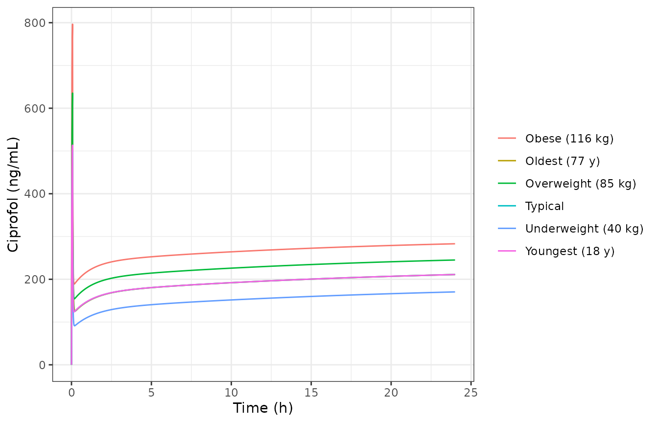
Replicates Figure S6 of Liu 2024: typical-value concentration-time profiles for the typical 33-year-old, 62 kg patient and the extreme ages and weights (left panel 0-24 h, right panel 0-20 min).
p2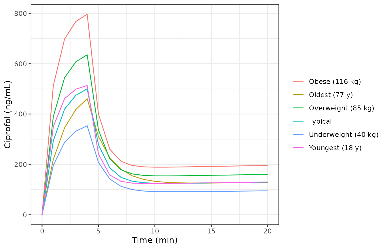
Replicates Figure S6 of Liu 2024: typical-value concentration-time profiles for the typical 33-year-old, 62 kg patient and the extreme ages and weights (left panel 0-24 h, right panel 0-20 min).
PKNCA validation
AUC0-24h and Cmax are computed with PKNCA from the typical-value profiles, one group per scenario.
nca_conc <- sim_typ |>
  filter(!is.na(Cc)) |>
  select(id, scenario, time, Cc)
# Time-zero guarantee (the observation grid already starts at 0).
nca_conc <- bind_rows(
  nca_conc,
  nca_conc |> distinct(id, scenario) |> mutate(time = 0, Cc = 0)
) |>
  distinct(id, scenario, time, .keep_all = TRUE) |>
  arrange(id, time)

nca_dose <- ev_typ |>
  filter(evid == 1) |>
  select(id, scenario, time, amt)

conc_obj <- PKNCA::PKNCAconc(nca_conc, Cc ~ time | scenario + id,
                             concu = "ng/mL", timeu = "h")
dose_obj <- PKNCA::PKNCAdose(nca_dose, amt ~ time | scenario + id, doseu = "mg")
intervals <- data.frame(start = 0, end = 24, cmax = TRUE, auclast = TRUE)
nca_res <- PKNCA::pk.nca(PKNCA::PKNCAdata(conc_obj, dose_obj, intervals = intervals))
nca_tbl <- as.data.frame(nca_res$result)
stopifnot(nrow(nca_tbl) == 2 * nrow(scenarios))
Comparison against published values
published <- tibble::tribble(
  ~scenario,               ~auclast, ~cmax,
  "Typical",                   4606, 500.3,
  "Youngest (18 y)",           4608, 513.7,
  "Oldest (77 y)",             4602, 461.0,
  "Underweight (40 kg)",       3638, 353.6,
  "Overweight (85 kg)",        5424, 635.3,
  "Obese (116 kg)",            6345, 796.5
)

cmp <- nlmixr2lib::ncaComparisonTable(
  simulated = nca_tbl |> filter(scenario %in% published$scenario),
  reference = published,
  by = "scenario",
  units = c(auclast = "ng*h/mL", cmax = "ng/mL"),
  tolerance_pct = 20
)
knitr::kable(cmp, caption = "Typical-value AUC0-24h and Cmax, simulated vs Liu 2024 Results 'Impact of body weight and age on exposure'. * differs from the reference by more than 20%.")| NCA parameter | scenario | Reference | Simulated | % diff |
|---|---|---|---|---|
| Cmax (ng/mL) | Typical | 500 | 500 | +0.0% |
| Cmax (ng/mL) | Youngest (18 y) | 514 | 514 | -0.0% |
| Cmax (ng/mL) | Oldest (77 y) | 461 | 461 | +0.0% |
| Cmax (ng/mL) | Underweight (40 kg) | 354 | 354 | -0.0% |
| Cmax (ng/mL) | Overweight (85 kg) | 635 | 635 | +0.0% |
| Cmax (ng/mL) | Obese (116 kg) | 796 | 796 | -0.0% |
| AUClast (ng*h/mL) | Typical | 4610 | 4610 | +0.0% |
| AUClast (ng*h/mL) | Youngest (18 y) | 4610 | 4610 | +0.0% |
| AUClast (ng*h/mL) | Oldest (77 y) | 4600 | 4600 | +0.0% |
| AUClast (ng*h/mL) | Underweight (40 kg) | 3640 | 3640 | +0.0% |
| AUClast (ng*h/mL) | Overweight (85 kg) | 5420 | 5430 | +0.0% |
| AUClast (ng*h/mL) | Obese (116 kg) | 6340 | 6350 | +0.0% |
check <- nca_tbl |>
  filter(scenario %in% published$scenario) |>
  select(scenario, PPTESTCD, Simulated = PPORRES) |>
  inner_join(
    published |> pivot_longer(-scenario, names_to = "PPTESTCD", values_to = "Reference"),
    by = c("scenario", "PPTESTCD")
  ) |>
  mutate(pct_diff = 100 * (Simulated - Reference) / Reference)

# Deterministic (zeroRe, fixed covariates): the only differences are rounding
# of the published parameters and the AUC integration, so a 1% bound is safe
# and still catches any mis-transcribed parameter or covariate effect.
stopifnot(
  nrow(check) == 12L,
  !anyNA(check$pct_diff),
  all(abs(check$pct_diff) < 1)
)
The covariate-sensitivity contrasts are expressed relative to the typical patient, exactly as the paper reports them.
sens <- nca_tbl |>
  select(scenario, PPTESTCD, PPORRES) |>
  pivot_wider(names_from = PPTESTCD, values_from = PPORRES) |>
  mutate(
    auc_pct = 100 * (auclast / auclast[scenario == "Typical"] - 1),
    cmax_pct = 100 * (cmax / cmax[scenario == "Typical"] - 1)
  ) |>
  filter(scenario %in% c("Non-ICU", "Venous sampling", "Female")) |>
  left_join(
    tibble::tribble(
      ~scenario,         ~pub_auc_pct, ~pub_cmax_pct,
      "Non-ICU",                 20.9,          8.97,
      "Venous sampling",         16.9,          7.43,
      "Female",                    NA,            NA
    ),
    by = "scenario"
  )

sens |>
  select(scenario, auc_pct, pub_auc_pct, cmax_pct, pub_cmax_pct) |>
  rename(
    "Scenario" = scenario,
    "AUC0-24h change, simulated (%)" = auc_pct,
    "AUC0-24h change, published (%)" = pub_auc_pct,
    "Cmax change, simulated (%)" = cmax_pct,
    "Cmax change, published (%)" = pub_cmax_pct
  ) |>
knitr::kable(digits = 2, caption = "Covariate sensitivity relative to the typical patient (Liu 2024 Results 'Covariate sensitivity analysis'; the paper gives only '< 7.1%' for sex).")| Scenario | AUC0-24h change, simulated (%) | AUC0-24h change, published (%) | Cmax change, simulated (%) | Cmax change, published (%) |
|---|---|---|---|---|
| Female | -7.09 | NA | -3.55 | NA |
| Non-ICU | 20.87 | 20.9 | 8.96 | 8.97 |
| Venous sampling | 16.96 | 16.9 | 7.43 | 7.43 |
stopifnot(
  abs(sens$auc_pct[sens$scenario == "Non-ICU"] - 20.9) < 0.5,
  abs(sens$cmax_pct[sens$scenario == "Non-ICU"] - 8.97) < 0.5,
  abs(sens$auc_pct[sens$scenario == "Venous sampling"] - 16.9) < 0.5,
  abs(sens$cmax_pct[sens$scenario == "Venous sampling"] - 7.43) < 0.5,
  # Female clearance is higher, so exposure falls, and by no more than 7.1%.
  sens$auc_pct[sens$scenario == "Female"] < 0,
  abs(sens$auc_pct[sens$scenario == "Female"]) < 7.15,
  abs(sens$cmax_pct[sens$scenario == "Female"]) < 7.15
)
Virtual ICU cohort
Figures 4 and 5 and Table S4 simulate the ICU sedation regimens in mechanically ventilated patients. The paper does not print the covariates of the simulated patients; the cohort below follows the ICU column of Table 1 (median weight 63.5 kg, range 42-90; median age 57 years, range 19-77; 39.3% female; 93.75% sampled arterially only) and holds the two study-level indicators at the ICU long-term-infusion levels.
The same 150 virtual patients receive every regimen, as in the paper
(its 0.2 mg/kg column of Table S4 is exactly twice its 0.1 mg/kg
column). Their random effects are drawn in base R from the model’s
omega and passed to the solver as parameters, so the cohort
does not depend on rxode2’s per-thread random-number streams.
set.seed(20240305)
n_per_arm <- 150

icu <- tibble(
  k = seq_len(n_per_arm),
  WT = pmin(pmax(rlnorm(n_per_arm, log(63.5), 0.17), 42), 90),
  AGE = pmin(pmax(round(rnorm(n_per_arm, 57, 14)), 19), 77),
  SEXF = rbinom(n_per_arm, 1, 0.393),
  SAMPLE_ARTERIAL = rbinom(n_per_arm, 1, 0.9375),
  DIS_CRITILL = 1,
  REGIMEN_CONTINF = 1
)
omega <- rxode2::rxode2(mod)$omega
#> ℹ parameter labels from comments will be replaced by 'label()'
eta <- matrix(rnorm(n_per_arm * nrow(omega)), n_per_arm) %*% chol(omega)
colnames(eta) <- rownames(omega)

arms_ld <- tidyr::expand_grid(ld_mgkg = c(0.1, 0.2), ld_min = c(0.5, 1, 2, 3, 4, 5)) |>
  mutate(md_mgkgh = 0.3, family = "Loading-dose duration")
arms_md <- tidyr::expand_grid(ld_mgkg = c(0.1, 0.2), md_mgkgh = c(0.06, 0.1, 0.2, 0.3, 0.8)) |>
  mutate(ld_min = 4, family = "Maintenance rate")
arms <- bind_rows(arms_ld, arms_md) |> mutate(arm = row_number())

md_dur <- 25  # h, Methods 'Target concentration'
ev_icu <- bind_rows(lapply(seq_len(nrow(arms)), function(i) {
  a <- arms[i, ]
  cov <- icu |> mutate(id = (i - 1L) * n_per_arm + k)
  ld_h <- a$ld_min / 60
  make_regimen(cov, a$ld_mgkg, ld_h, a$md_mgkgh, md_dur,
               sort(unique(c(seq(0, 25, by = 0.25), ld_h, ld_h + md_dur)))) |>
    mutate(arm = a$arm)
}))

stopifnot(all(table(ev_icu$arm[ev_icu$evid == 0]) > 0),
          length(unique(ev_icu$id)) == nrow(arms) * n_per_arm)

# One row of random effects per simulated id; patient k carries the same etas
# in every arm.
id_k <- distinct(ev_icu, id, k)
params <- data.frame(id = id_k$id, eta[id_k$k, , drop = FALSE])
Simulation
Individual predictions (Cc) are compared with the paper,
which reports model-predicted concentrations without residual error.
sim_icu <- rxode2::rxSolve(rxode2::zeroRe(mod), events = ev_icu, params = params,
                           returnType = "data.frame", keep = "arm") |>
  left_join(arms, by = "arm")
#> ℹ parameter labels from comments will be replaced by 'label()'
#> Warning: No sigma parameters in the model
#> Warning: multi-subject simulation without without 'omega'
Replicate published figures
target <- c(lo = 77.0, mid = 143.3, hi = 215.6)
fig4 <- sim_icu |>
  filter(family == "Loading-dose duration", ld_mgkg == 0.1) |>
  group_by(ld_min, time) |>
  summarise(med = median(Cc), lo = quantile(Cc, 0.05), hi = quantile(Cc, 0.95), .groups = "drop")
ggplot(fig4, aes(time, med)) +
  geom_ribbon(aes(ymin = lo, ymax = hi), fill = "steelblue", alpha = 0.25) +
  geom_line(colour = "steelblue") +
  geom_hline(yintercept = target["mid"], colour = "red") +
  geom_hline(yintercept = target[c("lo", "hi")], colour = "red", linetype = "dashed") +
  facet_wrap(~ paste("LD duration", ld_min, "min")) +
  labs(x = "Time (h)", y = "Ciprofol (ng/mL)") +
  theme_bw()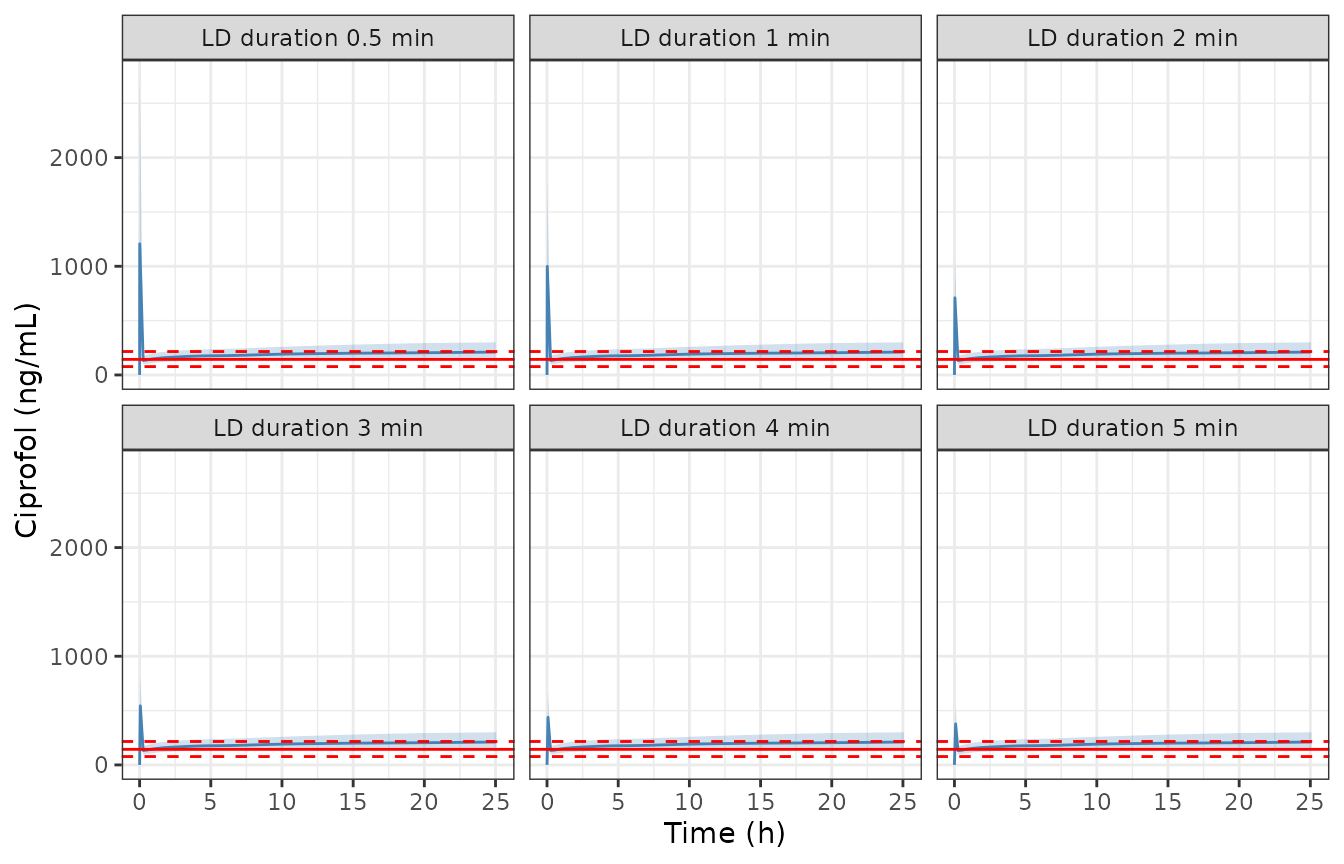
Replicates Figure 4 of Liu 2024: a 0.1 mg/kg loading dose over 0.5-5 min followed by 0.3 mg/kg/h (median and 5th-95th percentile of the individual predictions). Red lines: median and 5th-95th percentile of the target concentration (143.3; 77.0-215.6 ng/mL).
fig5 <- sim_icu |>
  filter(family == "Maintenance rate", ld_mgkg == 0.1, md_mgkgh <= 0.3) |>
  group_by(md_mgkgh, time) |>
  summarise(med = median(Cc), lo = quantile(Cc, 0.05), hi = quantile(Cc, 0.95), .groups = "drop")
ggplot(fig5, aes(time, med)) +
  geom_ribbon(aes(ymin = lo, ymax = hi), fill = "steelblue", alpha = 0.25) +
  geom_line(colour = "steelblue") +
  geom_hline(yintercept = target["mid"], colour = "red") +
  geom_hline(yintercept = target[c("lo", "hi")], colour = "red", linetype = "dashed") +
  facet_wrap(~ paste("MD", md_mgkgh, "mg/kg/h")) +
  labs(x = "Time (h)", y = "Ciprofol (ng/mL)") +
  theme_bw()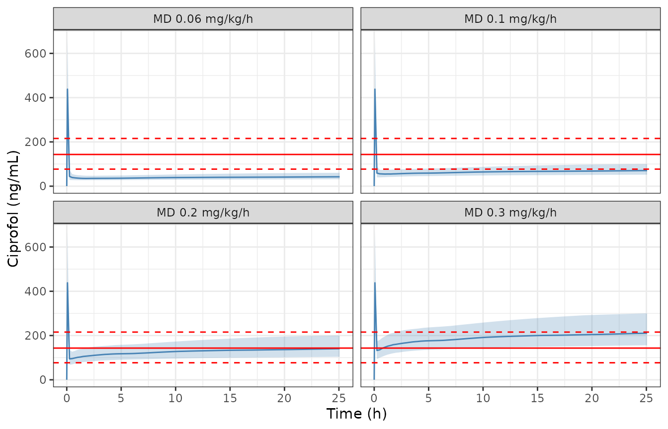
Replicates Figure 5 of Liu 2024: a 0.1 mg/kg loading dose over 4 min followed by 0.06-0.3 mg/kg/h (median and 5th-95th percentile of the individual predictions).
Concentration at the end of the loading dose (Table S4)
Table S4 prints the median simulated concentration at the end of the loading infusion. Two cells are defective in the source: the 0.5 min, 0.1 mg/kg median is printed as 127 ng/mL although its own ‘% change’ column (593% of the 215.6 ng/mL upper target) and the 0.2 mg/kg row (2556 ng/mL, twice the dose) both imply about 1278 ng/mL, and the 5 min, 0.2 mg/kg median is missing. Both are shown but not gated.
ld_end <- sim_icu |>
  filter(family == "Loading-dose duration", abs(time - ld_min / 60) < 1e-9) |>
  group_by(ld_mgkg, ld_min) |>
  summarise(Simulated = median(Cc), n = n(), .groups = "drop") |>
  left_join(
    tibble::tribble(
      ~ld_mgkg, ~ld_min, ~Published,
      0.1, 0.5,  NA,
      0.1, 1,  1059,
      0.1, 2,   732,
      0.1, 3,   572,
      0.1, 4,   464,
      0.1, 5,   388,
      0.2, 0.5, 2556,
      0.2, 1,  2119,
      0.2, 2,  1463,
      0.2, 3,  1143,
      0.2, 4,   928,
      0.2, 5,    NA
    ),
    by = c("ld_mgkg", "ld_min")
  ) |>
  mutate(pct_diff = 100 * (Simulated - Published) / Published)

ld_end |>
  rename("Loading dose (mg/kg)" = ld_mgkg, "Duration (min)" = ld_min,
         "Simulated median (ng/mL)" = Simulated, "Published median (ng/mL)" = Published,
         "% difference" = pct_diff, "Subjects" = n) |>
knitr::kable(digits = 1, caption = "Median concentration at the end of the loading-dose infusion, simulated vs Liu 2024 Table S4.")| Loading dose (mg/kg) | Duration (min) | Simulated median (ng/mL) | Subjects | Published median (ng/mL) | % difference |
|---|---|---|---|---|---|
| 0.1 | 0.5 | 1206.8 | 150 | NA | NA |
| 0.1 | 1.0 | 999.8 | 150 | 1059 | -5.6 |
| 0.1 | 2.0 | 710.4 | 150 | 732 | -3.0 |
| 0.1 | 3.0 | 544.0 | 150 | 572 | -4.9 |
| 0.1 | 4.0 | 438.4 | 150 | 464 | -5.5 |
| 0.1 | 5.0 | 377.8 | 150 | 388 | -2.6 |
| 0.2 | 0.5 | 2413.5 | 150 | 2556 | -5.6 |
| 0.2 | 1.0 | 1999.5 | 150 | 2119 | -5.6 |
| 0.2 | 2.0 | 1420.7 | 150 | 1463 | -2.9 |
| 0.2 | 3.0 | 1088.0 | 150 | 1143 | -4.8 |
| 0.2 | 4.0 | 876.7 | 150 | 928 | -5.5 |
| 0.2 | 5.0 | 755.5 | 150 | NA | NA |
gated <- filter(ld_end, !is.na(Published))
stopifnot(
  nrow(gated) == 10L,
  all(gated$n == n_per_arm),
  # Centre: a wrong V1, age effect or unit moves every row together.
  abs(median(gated$pct_diff)) < 10,
  # Envelope across rows, robust to which subjects land in the tails.
  quantile(abs(gated$pct_diff), 0.9) < 20
)
Concentration at the end of the maintenance infusion
md_end <- sim_icu |>
  filter(family == "Maintenance rate", abs(time - (ld_min / 60 + md_dur)) < 1e-9) |>
  group_by(ld_mgkg, md_mgkgh) |>
  summarise(Simulated = median(Cc), n = n(), .groups = "drop") |>
  left_join(
    tibble::tribble(
      ~ld_mgkg, ~md_mgkgh, ~Published,
      0.1, 0.06, 41.6,
      0.1, 0.1,  69.1,
      0.1, 0.2,   138,
      0.1, 0.3,   207,
      0.1, 0.8,   550,
      0.2, 0.06, 41.9,
      0.2, 0.1,  69.4,
      0.2, 0.2,   138,
      0.2, 0.3,   207,
      0.2, 0.8,   551
    ),
    by = c("ld_mgkg", "md_mgkgh")
  ) |>
  mutate(pct_diff = 100 * (Simulated - Published) / Published)

md_end |>
  mutate(md_mgkgh = as.character(md_mgkgh)) |>
  rename("Loading dose (mg/kg)" = ld_mgkg, "Maintenance (mg/kg/h)" = md_mgkgh,
         "Simulated median (ng/mL)" = Simulated, "Published (ng/mL)" = Published,
         "% difference" = pct_diff, "Subjects" = n) |>
knitr::kable(digits = 1, caption = "Concentration at the end of the 25 h maintenance infusion, simulated median vs Liu 2024 Results 'Target concentration interval'.")| Loading dose (mg/kg) | Maintenance (mg/kg/h) | Simulated median (ng/mL) | Subjects | Published (ng/mL) | % difference |
|---|---|---|---|---|---|
| 0.1 | 0.06 | 42.4 | 150 | 41.6 | 2.0 |
| 0.1 | 0.1 | 70.5 | 150 | 69.1 | 2.0 |
| 0.1 | 0.2 | 140.5 | 150 | 138.0 | 1.8 |
| 0.1 | 0.3 | 210.6 | 150 | 207.0 | 1.7 |
| 0.1 | 0.8 | 560.9 | 150 | 550.0 | 2.0 |
| 0.2 | 0.06 | 42.7 | 150 | 41.9 | 1.9 |
| 0.2 | 0.1 | 70.8 | 150 | 69.4 | 2.0 |
| 0.2 | 0.2 | 140.9 | 150 | 138.0 | 2.1 |
| 0.2 | 0.3 | 211.0 | 150 | 207.0 | 1.9 |
| 0.2 | 0.8 | 561.3 | 150 | 551.0 | 1.9 |
Assumptions and deviations
-
Direction of the sex effect. The Results text
states that “Women exhibited 9.31% lower CL compared to men”. Equation 3
(
+0.089 * sex = female), the Table 2 factor of 1.09 for female sex and the sex panel of Figure 1 all show female clearance 9.3% higher than male, and only that direction reproduces the sensitivity statement that sex changes exposure by less than 7.1% (the simulation above gives about -7.1% for AUC0-24h). The model follows the equation. - “35.1% lower” clearance in short-term non-ICU studies. The Results text says clearance was 35.1% lower in short-term infusion non-ICU studies than in long-term ICU studies. Equation 3 and Table 2 give exp(0.229 - 0.237) = 0.992 for that combination, essentially no difference, and the Figure 1 study-design panel shows short-term studies with higher clearance. 35.1% equals 1 - 0.789 x 0.823, the ICU factor multiplied by the venous-sampling factor, so the sentence appears to combine the wrong pair of effects. The model follows the equation.
-
Inverted indicator coding. The paper’s flags are
the complements of the package’s canonical covariates: its
ICUflag is 1 for the non-ICU studies,FLGis 1 for short-term infusion studies, andSITE0is 1 for venous samples. The model keeps the paper’s coefficients and signs and applies them to1 - DIS_CRITILL,1 - REGIMEN_CONTINFand1 - SAMPLE_ARTERIAL, so the typical values are those of an arterially sampled ICU patient in a long-term infusion study, as in the paper. -
Study design is a study-level flag.
REGIMEN_CONTINFfollows the paper’s per-study assignment (HSK3486-102, -204, -205, -306 and -307 are long-term infusion studies), not the duration of each individual dose. Its effects on V2 (x 0.125) and V3 (x 0.198) are large, so simulating a regimen that was not studied requires a choice of level; the ICU sedation simulations here use the long-term level. -
Sampling site is per record. In the NONMEM
$PKblock the venous flag changes clearance on each record, so a subject sampled at both sites has a clearance that switches between records. The model reproduces this whenSAMPLE_ARTERIALis supplied per observation row. The simulations above hold it constant per subject. -
IIV and residual magnitudes. Table 2 prints IIV and
residual variability in percent. The control stream’s
$OMEGAand$SIGMAvalues are the squares of those percentages to within the last digit, so the percentages are read as log-scale standard deviations and squared to give the variances. - ICU cohort. The covariates of the patients simulated for Figures 4 and 5 and Table S4 are not reported. The cohort above is drawn to match the ICU column of Table 1; its weight and age distributions are assumptions.
- Table S4 defects. Two cells of Table S4 are unusable (see above) and are not used in the gate.
- Exposure-safety analysis. The logistic regression of hypotension on exposure is described only as showing no clinically meaningful relationship, with no coefficients reported (“data not shown”), so there is no exposure-response model to encode.