Unecritinib and crizotinib (Yang 2021)

Model and source

• Citation: Yang F, Wu H, Bo Y, Lu Y, Pan H, Li S, Lu Q, Xie S, Liao H, Wang B. Population Pharmacokinetic Modeling and Simulation of TQ-B3101 to Inform Dosing in Pediatric Patients With Solid Tumors. Front Pharmacol. 2021;12:782518 (published 18 January 2022). doi:10.3389/fphar.2021.782518.
• Description: Joint parent-metabolite population PK model for the ALK/ROS1 kinase inhibitor unecritinib (TQ-B3101) and its active metabolite crizotinib (TQ-B3101M) in adults with advanced solid tumours and adolescents with relapsed or refractory ALK-positive anaplastic large cell lymphoma (Yang 2021). Unecritinib is described by a one-compartment model with first-order absorption and first-order elimination; all of its clearance forms crizotinib by amide hydrolysis (fraction metabolised fixed to 1 on a molar basis for identifiability), which is described by a two-compartment model whose apparent clearance decreases exponentially with time since the first dose, CLm(t) = CLm0 * (1 + famp * (1 - exp(-k * t))) with famp = -0.41, to a steady-state value 41 percent below the first-dose value. All clearances and volumes are apparent (X/F for the parent, X/Fm for the metabolite, i.e. proportional to the true metabolite values by the unknown fraction metabolised). No covariate was retained. The paper names the analytes only by development code and withholds their molecular weights; the maintainers identified them from PubChem and apply the crizotinib / unecritinib molecular-weight ratio to the formation flux so that Cc_crizotinib is in crizotinib mass units. Below-quantitation-limit samples were discarded (M1 method) in the source analysis.
• Article: https://doi.org/10.3389/fphar.2021.782518 (open access)

Unecritinib (development code TQ-B3101) is an oral ALK/ROS1/MET kinase inhibitor that is rapidly converted by amide hydrolysis to its active metabolite (TQ-B3101M). Yang 2021 fitted the two analytes sequentially in NONMEM 7.4 (FOCE-I): a one-compartment model with first-order absorption for the parent was fitted first and fixed, then a two-compartment model for the metabolite was added. All of the parent’s clearance forms the metabolite (the fraction metabolised, FM, was fixed to 1 for identifiability), and the metabolite’s apparent clearance falls exponentially with time since the first dose, by 41% at its asymptote (Table 3, footnote a). No covariate was retained.

Identity of the analytes

The paper refers to the two analytes only as TQ-B3101 and TQ-B3101M and states that “the information of TQ-B3101 and TQ-B3101M including structure, molecular formular and molecular weight cannot be provided due to a proprietary issue” (Methods, Analytical Methods). The identities are now public:

• PubChem CID 71506874, unecritinib, lists TQ-B3101 as a synonym: C23H24Cl2FN5O2, 492.4 g/mol, the N-acetyl amide of crizotinib.
• Hydrolysis of that amide gives crizotinib (PubChem CID 11626560, C21H22Cl2FN5O, 450.3 g/mol). Later bioanalytical work names crizotinib as the active metabolite of unecritinib (doi:10.1016/j.jpba.2024.116199).
• The paper’s own numbers agree. The Discussion equates 300 mg TQ-B3101 with 275 mg crizotinib, and its Eq. 4 converts crizotinib doses to TQ-B3101 doses by the molecular-weight ratio of the two. 275 / 300 = 0.917, and 450.3 / 492.4 = 0.914.

The data were fitted as molar concentrations: the LLOQ was 1 nmol/L for both analytes and the goodness-of-fit plots are in molar units. With FM fixed to 1, one mole of crizotinib therefore forms per mole of unecritinib cleared. The packaged model applies the molecular-weight ratio to the formation flux, so the metabolite states hold mg of crizotinib and Cc_crizotinib is in ng/mL of crizotinib. The paper’s paediatric Table 6 and adult exposures are in those units, and the comparisons below are direct.

Population

The analysis pooled 40 patients from two Chinese studies (Table 1): a Phase 1 dose-escalation study in adults with advanced solid tumours (NCT03019276; single doses of 100 or 200 mg, then 100, 200 or 300 mg once daily for 28 days) and a Phase 2 single-arm study in adults and adolescents with relapsed or refractory ALK-positive anaplastic large cell lymphoma (NCT04306887; 200, 250, 300 or 350 mg twice daily for 28 days). All doses were taken fasting. Table 2: 34 adults (median age 51.5 years, range 28-73; median weight 59.0 kg, range 42.0-87.7) and 6 adolescents (median age 13.0 years, range 11-14; median weight 41.8 kg, range 32.9-68.0); 21 of 40 (52.5%) were male. The dataset held 375 quantifiable unecritinib and 658 quantifiable crizotinib concentrations; the 340 and 42 below-quantitation samples were discarded.

The same information is available programmatically via readModelDb("Yang_2021_unecritinib")()$population.

Source trace

The per-parameter origin is recorded as an in-file comment next to each ini() entry in inst/modeldb/specificDrugs/Yang_2021_unecritinib.R.

Equation / parameter	Value	Source location
lcl (CL/F)	log(2850) L/h	Table 3
lvc (V/F)	log(4200) L	Table 3
lka (Ka)	log(51.9) 1/h	Table 3
fm (FM)	fixed(1)	Methods, Pharmacokinetic Modeling; Figure 1 caption
lcl_crizotinib (CLm0/Fm)	log(126) L/h	Table 3
lvc_crizotinib (Vcm/Fm)	log(2300) L	Table 3
lq_crizotinib (Qm/Fm)	log(113) L/h	Table 3
lvp_crizotinib (Vpm/Fm)	log(1480) L	Table 3
cl_exp_famp (-TDPK)	-0.41	Table 3 (TDPK = 0.41)
lcl_exp_kdes (KTDPK)	log(0.0363) 1/h	Table 3
etalcl, etalvc	0.0760, 0.1010	Table 3 (28.1, 32.6 %CV); omega^2 = log(1 + CV^2)
etalcl_crizotinib, etalvc_crizotinib, etalvp_crizotinib	0.1100, 0.2484, 0.5300	Table 3 (34.1, 53.1, 83.6 %CV)
propSd, propSd_crizotinib	0.711, 0.319	Table 3 (sigma 71.1, 31.9 %CV)
mw_unecritinib, mw_crizotinib	492.4, 450.3 g/mol	PubChem CIDs 71506874 and 11626560 (not in the paper)
theta_i = theta_TV * exp(eta_i)	n/a	Methods, Eq. 1
CLm(t) = CLm0 * [1 - TDPK * (1 - exp(-KTDPK * t))]	n/a	Table 3, footnote a
Parent -> metabolite -> two-compartment ODEs	n/a	Figure 1

Structural checks against the published half-lives

The Abstract and Results quote an elimination half-life of 1.0 h for unecritinib and, for the metabolite at steady state, distribution and elimination half-lives of 4.9 and 39.4 h. These follow in closed form from the typical values, using the asymptotic metabolite clearance CLm0 * (1 + cl_exp_famp).

mod <- readModelDb("Yang_2021_unecritinib")
th <- rxode2::rxode2(mod)$theta
#> ℹ parameter labels from comments will be replaced by 'label()'

cl_p <- exp(th[["lcl"]])
vc_p <- exp(th[["lvc"]])
cl_m_inf <- exp(th[["lcl_crizotinib"]]) * (1 + th[["cl_exp_famp"]])
vc_m <- exp(th[["lvc_crizotinib"]])
q_m <- exp(th[["lq_crizotinib"]])
vp_m <- exp(th[["lvp_crizotinib"]])

k10 <- cl_m_inf / vc_m
k12 <- q_m / vc_m
k21 <- q_m / vp_m
sum_k <- k10 + k12 + k21
root <- sqrt(sum_k^2 - 4 * k10 * k21)

hl <- tibble::tibble(
  Quantity = c(
    "Unecritinib elimination half-life (h)",
    "Crizotinib distribution half-life at steady state (h)",
    "Crizotinib elimination half-life at steady state (h)",
    "Crizotinib apparent clearance at steady state (L/h)"
  ),
  Model = c(
    log(2) * vc_p / cl_p,
    log(2) / ((sum_k + root) / 2),
    log(2) / ((sum_k - root) / 2),
    cl_m_inf
  ),
  Published = c(1.0, 4.9, 39.4, 126 * (1 - 0.41))
) |>
  mutate(`Difference (%)` = 100 * (Model / Published - 1))

knitr::kable(hl, digits = 2, caption = "Closed-form half-lives versus Yang 2021 (Abstract; Results).")

Closed-form half-lives versus Yang 2021 (Abstract; Results).

Quantity	Model	Published	Difference (%)
Unecritinib elimination half-life (h)	1.02	1.00	2.15
Crizotinib distribution half-life at steady state (h)	4.94	4.90	0.90
Crizotinib elimination half-life at steady state (h)	39.38	39.40	-0.05
Crizotinib apparent clearance at steady state (L/h)	74.34	74.34	0.00

# Deterministic identities of the typical values; the published half-lives are
# printed to one decimal, so each must agree to within that rounding (<= 3%).
stopifnot(all(abs(hl$`Difference (%)`) < 3))

Time course of the metabolite clearance

tc <- tibble::tibble(time = seq(0, 240, by = 1)) |>
  mutate(cl_crizotinib = exp(th[["lcl_crizotinib"]]) *
    (1 + th[["cl_exp_famp"]] * (1 - exp(-exp(th[["lcl_exp_kdes"]]) * time))))

ggplot(tc, aes(time / 24, cl_crizotinib)) +
  geom_line() +
  geom_hline(yintercept = cl_m_inf, linetype = "dashed") +
  labs(
    x = "Time since first dose (days)", y = "CLm/Fm (L/h)",
    title = "Typical crizotinib apparent clearance after unecritinib dosing",
    caption = "Table 3 footnote a of Yang 2021; dashed line = asymptote 74.3 L/h."
  )

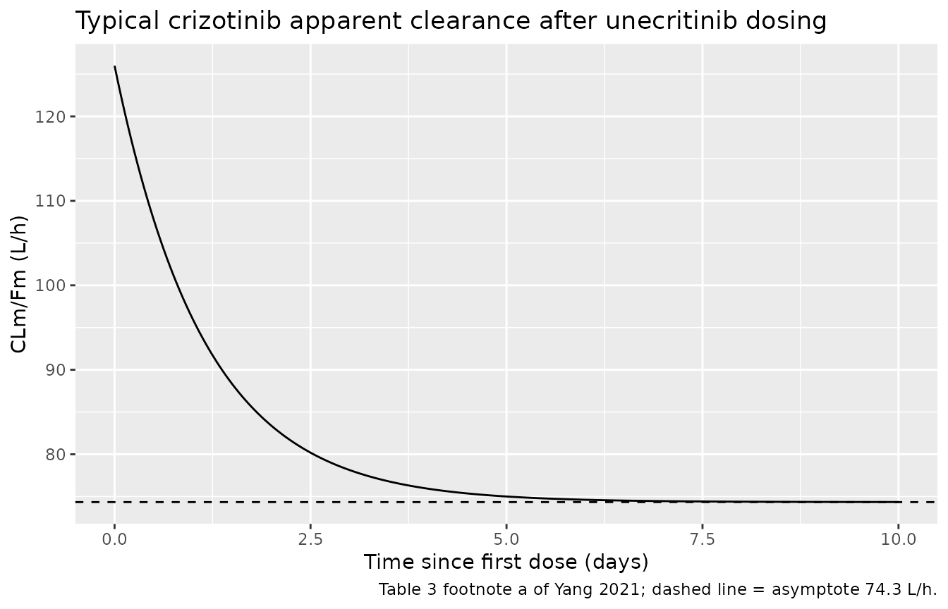
The half-time of the decline is log(2) / 0.0363 = 19.1 h, so the clearance is within 1% of its asymptote after about 5.3 days. The authors attribute the decline to auto-inhibition of CYP3A4, as reported for crizotinib given as crizotinib, whose mean CL/F falls from 100 L/h after a single dose to 60 L/h at steady state (Discussion).

Typical-value simulation and a steady-state identity

mod_typ <- rxode2::zeroRe(mod)
#> ℹ parameter labels from comments will be replaced by 'label()'
mw_ratio <- 450.3 / 492.4

ev_typ <- rxode2::et(amt = 300, cmt = "depot", ii = 12, addl = 55) |>
  rxode2::et(sort(unique(c(seq(0, 48, by = 0.1), seq(648, 672, by = 0.05)))), cmt = "central") |>
  as.data.frame() |>
  # Two residual-error endpoints: observation rows carry dvid = 1; a forward
  # solve still returns both Cc and Cc_crizotinib on every row.
  mutate(dvid = ifelse(evid == 0, 1L, NA_integer_))
sim_typ <- rxode2::rxSolve(mod_typ, ev_typ, rtol = 1e-10, atol = 1e-12) |>
  as.data.frame()
#> ℹ omega/sigma items treated as zero: 'etalcl', 'etalvc', 'etalcl_crizotinib', 'etalvc_crizotinib', 'etalvp_crizotinib'

# At true steady state AUC0-tau of the metabolite equals
# fm * dose * MW ratio / CLm(inf) (the clearance has relaxed to within 1e-10 of
# its asymptote by day 28).
last <- sim_typ |> filter(time >= 660, time <= 672)
auc_num <- sum(diff(last$time) *
  (head(last$Cc_crizotinib, -1) + tail(last$Cc_crizotinib, -1)) / 2)
auc_closed <- 1000 * 300 * mw_ratio / cl_m_inf
c(numeric = auc_num, closed_form = auc_closed)
#>     numeric closed_form 
#>    3690.443    3690.478
# Solve against its own closed form: a pure numerical-error comparison.
# Trapezoidal error on the 0.05 h grid is ~1e-5 relative.
stopifnot(abs(auc_num / auc_closed - 1) < 1e-3)

sim_typ |>
  filter(time <= 48 | time >= 648) |>
  mutate(window = ifelse(time <= 48, "First two days", "Day 28 (steady state)")) |>
  select(time, window, Unecritinib = Cc, Crizotinib = Cc_crizotinib) |>
  pivot_longer(-c(time, window), names_to = "analyte", values_to = "conc") |>
  filter(conc > 0) |>
  ggplot(aes(time, conc, colour = analyte)) +
  geom_line() +
  facet_wrap(~window, scales = "free_x") +
  scale_y_log10() +
  labs(
    x = "Time (h)", y = "Concentration (ng/mL)", colour = NULL,
    title = "Typical profiles, 300 mg unecritinib twice daily"
  ) +
  theme(legend.position = "bottom")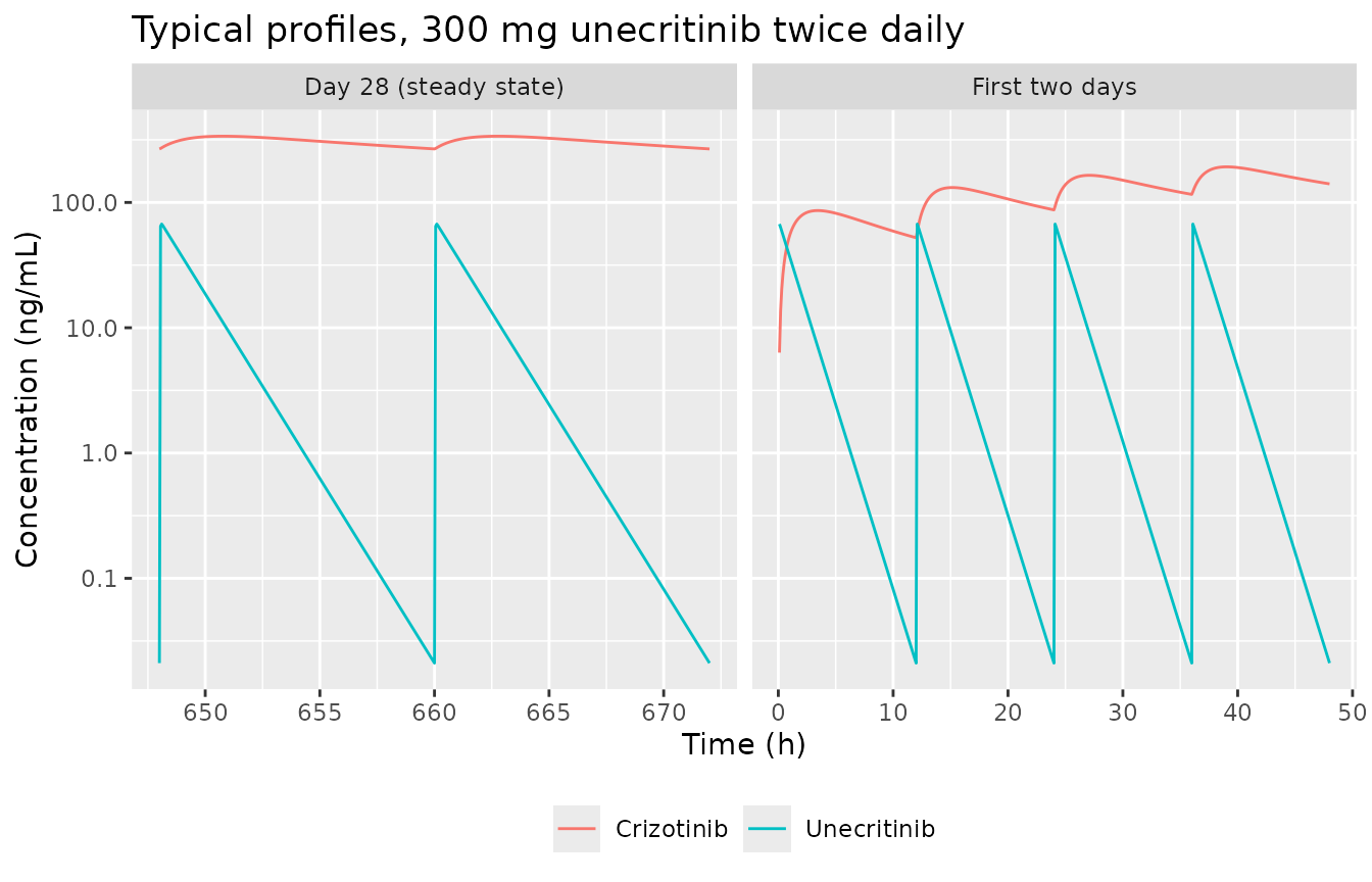

The parent peaks within an hour and is essentially gone before the next dose (half-life 1 h), while crizotinib peaks 1-3 h after the dose and accumulates, consistent with the times to peak of 0.5-1 h and 1-3 h quoted in the Discussion.

Virtual adult cohorts

Original observed data are not available. Each regimen below is a separate arm of 100 virtual patients who start at their first dose (the model’s time-varying clearance is indexed to time since the first dose). The model has no covariates, so no demographic distribution is needed.

rxode2::rxSetSeed(20211)

make_arm <- function(n, regimen, amt, ii, n_doses, obs, id_offset) {
  ids <- id_offset + seq_len(n)
  dose_times <- (seq_len(n_doses) - 1) * ii
  dose <- tidyr::expand_grid(id = ids, time = dose_times) |>
    mutate(evid = 1L, amt = amt, cmt = "depot")
  obs_rows <- tidyr::expand_grid(id = ids, time = obs) |>
    mutate(evid = 0L, amt = 0, cmt = "central", dvid = 1L)
  bind_rows(dose, obs_rows) |>
    mutate(regimen = regimen) |>
    arrange(id, time, desc(evid))
}

obs_sd <- c(0, 0.25, 0.5, 0.75, 1, 1.5, 2, 3, 4, 6, 8, 12, 24, 48, 72, 96, 144, 192, 240, 336)
obs_qd <- 648 + c(0, 0.25, 0.5, 0.75, 1, 1.5, 2, 3, 4, 6, 8, 12, 16, 24)
obs_bid <- 660 + c(0, 0.25, 0.5, 0.75, 1, 1.5, 2, 3, 4, 6, 8, 10, 12)

events <- bind_rows(
  make_arm(100, "100 mg single dose", 100, 24, 1, obs_sd, 0L),
  make_arm(100, "200 mg single dose", 200, 24, 1, obs_sd, 100L),
  make_arm(100, "100 mg QD, day 28", 100, 24, 28, obs_qd, 200L),
  make_arm(100, "200 mg QD, day 28", 200, 24, 28, obs_qd, 300L),
  make_arm(100, "300 mg BID, day 28", 300, 12, 56, obs_bid, 400L)
)
stopifnot(!anyDuplicated(unique(events[, c("id", "time", "evid")])))

sim <- rxode2::rxSolve(mod, events = events, keep = "regimen") |>
  as.data.frame()
#> ℹ parameter labels from comments will be replaced by 'label()'

PKNCA: accumulation of crizotinib

The Methods report that in the Phase 1 study “the average AUC0-tau,ss of TQ-B3101M after repeated dosing was 20-40% higher than the average AUC0-inf of TQ-B3101M after a single dose” at 100 and 200 mg. With linear kinetics and a constant clearance those two AUCs would be equal; the excess is produced by the time-dependent clearance, so it is the most direct check of that part of the model.

nca_input <- function(sim, analyte) {
  d <- sim |>
    filter(!is.na(.data[[analyte]])) |>
    transmute(id, time, regimen, Cc = pmax(.data[[analyte]], 0))
  # Time-zero rows for the single-dose arms (pre-dose concentration 0).
  bind_rows(
    d,
    d |> filter(grepl("single", regimen)) |> distinct(id, regimen) |>
      mutate(time = 0, Cc = 0)
  ) |>
    distinct(id, regimen, time, .keep_all = TRUE) |>
    arrange(id, regimen, time)
}

dose_df <- events |>
  filter(evid == 1) |>
  select(id, time, amt, regimen)

intervals <- data.frame(
  regimen = c(
    "100 mg single dose", "200 mg single dose", "100 mg QD, day 28",
    "200 mg QD, day 28", "300 mg BID, day 28"
  ),
  start = c(0, 0, 648, 648, 660),
  end = c(Inf, Inf, 672, 672, 672),
  cmax = TRUE,
  tmax = TRUE,
  aucinf.obs = c(TRUE, TRUE, FALSE, FALSE, FALSE),
  auclast = c(FALSE, FALSE, TRUE, TRUE, TRUE)
)

run_nca <- function(analyte) {
  conc <- PKNCA::PKNCAconc(nca_input(sim, analyte), Cc ~ time | regimen + id)
  dose <- PKNCA::PKNCAdose(dose_df, amt ~ time | regimen + id)
  PKNCA::pk.nca(PKNCA::PKNCAdata(conc, dose, intervals = intervals))
}

nca_m <- run_nca("Cc_crizotinib")
nca_p <- run_nca("Cc")

auc_by_subject <- as.data.frame(nca_m$result) |>
  filter(PPTESTCD %in% c("aucinf.obs", "auclast")) |>
  select(regimen, id, PPORRES)

acc <- auc_by_subject |>
  mutate(
    dose = ifelse(grepl("^100", regimen), "100 mg", "200 mg"),
    type = ifelse(grepl("single", regimen), "single", "repeated")
  ) |>
  filter(!grepl("BID", regimen)) |>
  group_by(dose, type) |>
  summarise(mean_auc = mean(PPORRES, na.rm = TRUE), .groups = "drop") |>
  pivot_wider(names_from = type, values_from = mean_auc) |>
  mutate(excess = 100 * (repeated / single - 1))

acc |>
  rename(
    "Unecritinib dose" = dose,
    "Mean single-dose crizotinib AUC0-inf (ng*h/mL)" = single,
    "Mean day-28 crizotinib AUC0-24 (ng*h/mL)" = repeated,
    "Excess (%)" = excess
  ) |>
  knitr::kable(digits = 1, caption = "Repeated-dose versus single-dose crizotinib exposure (published: 20-40% higher).")

Repeated-dose versus single-dose crizotinib exposure (published: 20-40% higher).

Unecritinib dose	Mean day-28 crizotinib AUC0-24 (ng*h/mL)	Mean single-dose crizotinib AUC0-inf (ng*h/mL)	Excess (%)
100 mg	1242.6	1048.9	18.5
200 mg	2709.1	2220.3	22.0

# Each per-dose excess compares two independent 100-subject means and carries
# ~7 percentage points of cohort noise, so only the pooled excess is gated
# here, with a bound a constant clearance (0%) or a mis-signed amplitude
# (negative) fails by several standard errors. The tight check is the
# deterministic typical-value excess below.
stopifnot(mean(acc$excess) > 0, mean(acc$excess) < 60)

# Typical-value excess: day-28 AUC0-24 = dose * MW ratio / CLm(inf) against
# the single-dose AUC0-inf of the typical subject (dense grid, numeric solve).
ev_sd <- rxode2::et(amt = 100, cmt = "depot") |>
  rxode2::et(c(seq(0, 24, by = 0.05), seq(24.5, 2000, by = 0.5)), cmt = "central") |>
  as.data.frame() |>
  mutate(dvid = ifelse(evid == 0, 1L, NA_integer_))
sd_typ <- rxode2::rxSolve(mod_typ, ev_sd, rtol = 1e-10, atol = 1e-12) |>
  as.data.frame()
#> ℹ omega/sigma items treated as zero: 'etalcl', 'etalvc', 'etalcl_crizotinib', 'etalvc_crizotinib', 'etalvp_crizotinib'
auc_sd_typ <- sum(diff(sd_typ$time) *
  (head(sd_typ$Cc_crizotinib, -1) + tail(sd_typ$Cc_crizotinib, -1)) / 2)
typ_excess <- 100 * ((1000 * 100 * mw_ratio / cl_m_inf) / auc_sd_typ - 1)
typ_excess
#> [1] 27.42467
# Deterministic: must fall in the 20-40% the Methods report.
stopifnot(typ_excess > 20, typ_excess < 40)

The simulated excess of repeated-dose over single-dose crizotinib exposure is 18% and 22% at 100 and 200 mg, against the 20-40% the paper reports from the Phase 1 non-compartmental analysis. The typical-value excess, free of cohort noise, is 27%, inside the published range; the per-dose cohort values scatter around it by the sampling noise of two independent 100-subject arms.

Adult steady-state exposure

The Discussion quotes a crizotinib (TQ-B3101M) AUC0-12h,ss of 4,251 ngh/mL after 300 mg unecritinib twice daily, against 3,880 ngh/mL after 250 mg crizotinib twice daily. The paper does not say whether 4,251 ng*h/mL is an observed mean from the Phase 2 patients or a model prediction, nor on which day.

published_adult <- tibble::tibble(regimen = "300 mg BID, day 28", auclast = 4251)

adult_res <- nca_m
adult_res$result <- adult_res$result |> filter(regimen == "300 mg BID, day 28")

cmp_adult <- nlmixr2lib::ncaComparisonTable(
  simulated = adult_res,
  reference = published_adult,
  by = "regimen",
  params = "auclast",
  units = c(auclast = "ng*h/mL"),
  tolerance_pct = 20
)
knitr::kable(cmp_adult, caption = "Crizotinib AUC0-12h,ss after 300 mg unecritinib BID: simulated median versus the Discussion value. * differs by >20%.")

Crizotinib AUC0-12h,ss after 300 mg unecritinib BID: simulated median versus the Discussion value. * differs by >20%.

NCA parameter	regimen	Reference	Simulated	% diff
AUClast (ng*h/mL)	300 mg BID, day 28	4250	3450	-18.8%

adult_sim_auc <- auc_by_subject$PPORRES[auc_by_subject$regimen == "300 mg BID, day 28"]
c(median = median(adult_sim_auc), mean = mean(adult_sim_auc))
#>   median     mean 
#> 3450.278 3603.853

The simulated median is 19% and the simulated mean 15% below the quoted value; the typical-value steady-state AUC, from the closed form above, is 3690 ngh/mL. The paper gives neither the source nor the sample size behind 4,251 ngh/mL, so the difference is recorded here rather than investigated further; it is not used to adjust the model.

Unecritinib (parent) NCA

as.data.frame(nca_p$result) |>
  filter(PPTESTCD %in% c("cmax", "tmax", "aucinf.obs", "auclast")) |>
  group_by(regimen, PPTESTCD) |>
  summarise(median = median(PPORRES, na.rm = TRUE), .groups = "drop") |>
  pivot_wider(names_from = PPTESTCD, values_from = median) |>
  knitr::kable(digits = 2, caption = "Median simulated unecritinib NCA parameters by regimen (the paper reports no parent NCA values to compare).")

Median simulated unecritinib NCA parameters by regimen (the paper reports no parent NCA values to compare).

regimen	auclast	cmax	tmax	aucinf.obs
100 mg QD, day 28	30.80	19.74	0.25	NA
100 mg single dose	NA	19.33	0.25	30.91
200 mg QD, day 28	65.38	40.00	0.25	NA
200 mg single dose	NA	39.69	0.25	63.75
300 mg BID, day 28	98.04	60.23	0.25	NA

Replicates Table 6 and Figure 4: paediatric BSA-tiered dosing

The paper’s paediatric simulation is not part of the fitted model. It applied body-weight allometry with fixed exponents of 0.75 on every clearance and 1 on every volume, “scaled to a median weight of adult patients” (Methods, Clinical Simulations). The median adult weight in Table 2 is 59.0 kg. The reference weight is not otherwise stated; 59.0 kg is used here. The allometric lines are added to a copy of the model inside this article only.

mod_ped <- mod |>
  rxode2::model({
    cl <- exp(lcl + etalcl) * (WT / 59)^0.75
    vc <- exp(lvc + etalvc) * (WT / 59)
    cl_crizotinib0 <- exp(lcl_crizotinib + etalcl_crizotinib) * (WT / 59)^0.75
    vc_crizotinib <- exp(lvc_crizotinib + etalvc_crizotinib) * (WT / 59)
    q_crizotinib <- exp(lq_crizotinib) * (WT / 59)^0.75
    vp_crizotinib <- exp(lvp_crizotinib + etalvp_crizotinib) * (WT / 59)
  })
#> ℹ parameter labels from comments will be replaced by 'label()'
#> ℹ add covariate `WT`

The paper’s 1,000 virtual children aged 6 to under 18 years came from the PK-Sim Asian population database (Table 4: median weight 42.3 kg, range 15.8-102.3; median BSA 1.3 m^2, range 0.7-2.2). That database is not reproduced here. Instead, BSA was drawn from a normal distribution with mean 1.3 m^2 and SD 0.3 m^2 truncated to 0.74-2.2 m^2 (the Table 4 median, and a spread whose +/-3 SD spans the Table 4 range), the first 100 children falling in each BSA tier of Table 5 were kept, and body weight was obtained by inverting the weight-only paediatric BSA formula of Costeff (1966), BSA = (4 WT + 7) / (WT + 90). That formula maps Table 4’s median weight of 42.3 kg to 1.33 m^2 and its weight range to 0.66-2.16 m^2, close to the tabulated BSA summary.

tiers <- tibble::tibble(
  tier = c("0.74-0.89", "0.90-1.22", "1.23-1.38", "1.39-1.59", ">1.6"),
  dose = c(250, 350, 400, 450, 550)
)

obs_ped <- 13 * 24 + c(0, 0.5, 1, 2, 4, 6, 10, 12) # Methods sampling grid, day 14

set.seed(20212)
bsa_pool <- rnorm(20000, mean = 1.3, sd = 0.3)
bsa_pool <- bsa_pool[bsa_pool >= 0.74 & bsa_pool <= 2.2]
ped_subjects <- tibble::tibble(
  BSA = bsa_pool,
  # Table 5 tiers are printed with gaps (0.89 | 0.90, 1.59 | 1.6); split them
  # at the midpoints.
  tier = as.character(cut(BSA, c(0.74, 0.895, 1.225, 1.385, 1.595, 2.2),
    labels = tiers$tier, include.lowest = TRUE
  ))
) |>
  group_by(tier) |>
  slice_head(n = 100) |>
  ungroup() |>
  left_join(tiers, by = "tier") |>
  mutate(
    id = seq_len(n()),
    WT = (90 * BSA - 7) / (4 - BSA)
  )
stopifnot(all(table(ped_subjects$tier) == 100L))

ped_events <- bind_rows(
  tidyr::expand_grid(ped_subjects, time = seq(0, 13 * 24, by = 12)) |>
    mutate(evid = 1L, amt = dose, cmt = "depot"),
  tidyr::expand_grid(ped_subjects, time = obs_ped) |>
    mutate(evid = 0L, amt = 0, cmt = "central", dvid = 1L)
) |>
  arrange(id, time, desc(evid))
stopifnot(!anyDuplicated(unique(ped_events[, c("id", "time", "evid")])))

rxode2::rxSetSeed(20213)
ped_sim <- rxode2::rxSolve(mod_ped, events = ped_events, keep = c("tier", "BSA")) |>
  as.data.frame()

ped_conc <- ped_sim |>
  filter(!is.na(Cc_crizotinib)) |>
  transmute(id, tier, time, Cc = pmax(Cc_crizotinib, 0))
ped_dose <- ped_events |>
  filter(evid == 1) |>
  select(id, tier, time, amt)
ped_nca <- PKNCA::pk.nca(PKNCA::PKNCAdata(
  PKNCA::PKNCAconc(ped_conc, Cc ~ time | tier + id),
  PKNCA::PKNCAdose(ped_dose, amt ~ time | tier + id),
  intervals = data.frame(start = 13 * 24, end = 13 * 24 + 12, cmax = TRUE, auclast = TRUE)
))

# Table 6 medians (the comparison table pools the simulation by median).
table6_median <- tibble::tibble(
  tier = tiers$tier,
  cmax = c(631.1, 620.8, 586.0, 597.7, 589.6),
  auclast = c(6583.9, 6507.4, 6259.7, 6376.8, 6379.0)
)

cmp_ped <- nlmixr2lib::ncaComparisonTable(
  simulated = ped_nca,
  reference = table6_median,
  by = "tier",
  params = c("cmax", "auclast"),
  units = c(cmax = "ng/mL", auclast = "ng*h/mL"),
  tolerance_pct = 20
)
knitr::kable(cmp_ped, caption = "Replicates Table 6 of Yang 2021: median crizotinib Cmax,ss and AUC0-12h,ss by BSA tier after BSA-tiered unecritinib dosing. * differs by >20%.")

Replicates Table 6 of Yang 2021: median crizotinib Cmax,ss and AUC0-12h,ss by BSA tier after BSA-tiered unecritinib dosing. * differs by >20%.

NCA parameter	tier	Reference	Simulated	% diff
Cmax (ng/mL)	0.74-0.89	631	636	+0.8%
Cmax (ng/mL)	0.90-1.22	621	703	+13.3%
Cmax (ng/mL)	1.23-1.38	586	594	+1.3%
Cmax (ng/mL)	1.39-1.59	598	605	+1.3%
Cmax (ng/mL)	>1.6	590	542	-8.1%
AUClast (ng*h/mL)	0.74-0.89	6580	6690	+1.6%
AUClast (ng*h/mL)	0.90-1.22	6510	7390	+13.6%
AUClast (ng*h/mL)	1.23-1.38	6260	6280	+0.4%
AUClast (ng*h/mL)	1.39-1.59	6380	6500	+2.0%
AUClast (ng*h/mL)	>1.6	6380	5870	-8.0%

ped_ind <- as.data.frame(ped_nca$result) |>
  filter(PPTESTCD %in% c("cmax", "auclast")) |>
  select(id, tier, PPTESTCD, PPORRES) |>
  pivot_wider(names_from = PPTESTCD, values_from = PPORRES)

ped_check <- ped_ind |>
  group_by(tier) |>
  summarise(sim_auc = median(auclast), sim_cmax = median(cmax), .groups = "drop") |>
  left_join(rename(table6_median, pub_auc = auclast, pub_cmax = cmax), by = "tier") |>
  mutate(
    pct_auc = 100 * (sim_auc / pub_auc - 1),
    pct_cmax = 100 * (sim_cmax / pub_cmax - 1)
  )
stopifnot(nrow(ped_check) == 5L, !anyNA(ped_check$pub_auc))
ped_check
#> # A tibble: 5 × 7
#>   tier      sim_auc sim_cmax pub_cmax pub_auc pct_auc pct_cmax
#>   <chr>       <dbl>    <dbl>    <dbl>   <dbl>   <dbl>    <dbl>
#> 1 0.74-0.89   6692.     636.     631.   6584.   1.64     0.784
#> 2 0.90-1.22   7389.     703.     621.   6507.  13.6     13.3  
#> 3 1.23-1.38   6285.     594.     586    6260.   0.400    1.31 
#> 4 1.39-1.59   6503.     605.     598.   6377.   1.97     1.26 
#> 5 >1.6        5868.     542.     590.   6379   -8.01    -8.14

# Structural: the BSA-tiered doses were chosen to give flat exposure, and the
# published tier medians span only 5%. Without the weight scaling the tiers
# would span 2.2-fold (250 to 550 mg). The simulated span is wider than the
# published one (realised 1.26 here, and 1.33 with a uniform-in-tier BSA draw)
# because weight is derived from BSA by the Costeff formula rather than drawn
# with height from PK-Sim, which shifts the within-tier weights; each tier
# median also carries ~4% sampling error. 1.5 sits outside that range and
# still fails a model without the allometric scaling.
stopifnot(max(ped_check$sim_auc) / min(ped_check$sim_auc) < 1.5)
# Level: a mis-transcribed clearance, a dropped molecular-weight ratio (-9%
# is inside the noise, but a mg/ng or molar slip is orders of magnitude) or a
# wrong reference weight moves every tier together.
stopifnot(abs(median(ped_check$pct_auc)) < 12, abs(median(ped_check$pct_cmax)) < 15)

ped_ind |>
  mutate(tier = factor(tier, levels = tiers$tier)) |>
  pivot_longer(c(cmax, auclast), names_to = "metric", values_to = "value") |>
  mutate(metric = ifelse(metric == "cmax", "Cmax,ss (ng/mL)", "AUC0-12h,ss (ng*h/mL)")) |>
  ggplot(aes(tier, value)) +
  geom_boxplot(outlier.size = 0.5) +
  geom_hline(
    data = tibble::tibble(
      metric = c("Cmax,ss (ng/mL)", "AUC0-12h,ss (ng*h/mL)"),
      ref = c(621, 6530)
    ),
    aes(yintercept = ref), linetype = "dashed"
  ) +
  facet_wrap(~metric, scales = "free_y") +
  labs(
    x = "BSA tier (m^2)", y = "Crizotinib",
    title = "Paediatric crizotinib exposure after BSA-tiered unecritinib dosing",
    caption = paste(
      "Replicates Figure 4 of Yang 2021. Dashed lines: crizotinib target",
      "exposure after the paediatric crizotinib label dose (Table 6)."
    )
  )

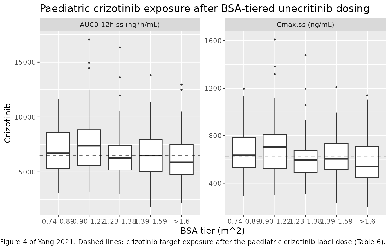
The simulated tier medians agree with the Table 6 medians to within 14%, with a median difference across tiers of 1.6% for AUC, and sit near the crizotinib target exposure the tiered regimen was designed to match (geometric-mean Cmax,ss 621 ng/mL, AUC0-12h,ss 6,530 ng*h/mL). The allometric bridge, the tiered doses and the molecular-weight conversion therefore reproduce the paper’s dosing simulation. The tier-to-tier pattern is less flat than in Table 6. The virtual children here get their weights from BSA through the Costeff formula, not from the PK-Sim population the paper used, and that moves the within-tier weights, most visibly in the wide 0.90-1.22 m^2 tier.

Assumptions and deviations

• Analyte identity and units. The paper withholds the structures and molecular weights. The maintainers identified TQ-B3101 as unecritinib and TQ-B3101M as crizotinib from PubChem and later literature, and took the molecular weights (492.4 and 450.3 g/mol) from PubChem. The model applies their ratio to the formation flux because the source fitted molar data with a molar fraction metabolised of 1. That choice is supported by the paper’s own 300 mg ~ 275 mg dose equivalence and by the Table 6 replication above. It is not a fitted value.
• Time-dependent clearance sign convention. The paper’s TDPK = 0.41 is a positive “maximum fraction reduction”. The model encodes it as the signed fractional amplitude cl_exp_famp = -0.41 in CLm(t) = CLm0 * (1 + cl_exp_famp * (1 - exp(-KTDPK * t))), which is algebraically identical and follows the sign convention of kel_exp_famp (negative = decline). Time t is time since the first dose, so simulations must start at the first dose. A washout between a single-dose and a repeated-dose period, as in the Phase 1 design, is not modelled as a reset of the clearance.
• IIV conversion. Table 3 reports IIV as %CV; variances were computed as omega^2 = log(1 + CV^2). No correlations are reported, so the etas are independent. Ka and Qm/Fm carry no IIV.
• BQL handling. The final model used the M1 method (below-quantitation samples discarded) for both analytes. The paper also evaluated M3 for the parent but reports only one set of estimates.
• Paediatric simulation. The allometric exponents (0.75 / 1), the reference weight (59.0 kg, the adult median of Table 2) and the BSA-tiered doses come from the paper’s simulation, not from the fitted model, which retained no covariate. The PK-Sim population the paper used is not available. The virtual children were therefore drawn from a truncated normal BSA distribution matching Table 4, and their weights derived from the Costeff
  1966. BSA formula. Steady state was taken on day 14, after the clearance has settled, because the paper does not state the day.
• Adult cohort. The accumulation check uses separate virtual arms for the single-dose and repeated-dose regimens, each starting at its own first dose.
• No erratum or correction notice for Yang 2021 was found in Crossref or Europe PMC as of 2026-09-30.