Model and source
mod_meta <- nlmixr2est::nlmixr(readModelDb("Lamoth_2009_imipenem"))$meta
#> ℹ parameter labels from comments will be replaced by 'label()'- Citation: Lamoth F, Buclin T, Csajka C, Pascual A, Calandra T, Marchetti O. Reassessment of recommended imipenem doses in febrile neutropenic patients with hematological malignancies. Antimicrob Agents Chemother. 2009;53(2):785-787. doi:10.1128/AAC.00891-08.
- Description: One-compartment IV population PK model for imipenem in adult febrile neutropenic patients with hematological malignancies (Lamoth 2009). Total clearance is the additive sum of a non-renal arm and a renal arm linear in Cockcroft-Gault GFR; the central volume of distribution scales linearly with total body weight referenced to 70 kg. A single log-normal inter-individual variability term is applied multiplicatively to the total clearance (TVCL = CL_nonren + CL_renal * GFR / 100), and residual error is proportional.
- Article (DOI): https://doi.org/10.1128/AAC.00891-08
This vignette validates the packaged
Lamoth_2009_imipenem model – a one-compartment IV
population PK model for imipenem in 57 adult febrile neutropenic
patients with hematological malignancies – against the source
publication’s Table 1 (baseline demographics and observed peak / trough
concentrations), Table 2 (final population PK model parameter
estimates), Figure 1 (simulated MIC90 coverage by dosing schedule), and
the post-hoc individual half-life summary reported in the Results.
Population
Lamoth 2009 retrospectively analyzed 159 plasma imipenem concentrations (86 troughs and 73 peaks) measured in 57 febrile neutropenic adults receiving imipenem at the Centre Hospitalier Universitaire Vaudois (Lausanne, Switzerland). The cohort was predominantly male (77.2% men, 22.8% women) with a median age of 58 years (range 17-78). Underlying hematological diseases were acute myeloid leukemia (64.9%), lymphoma (8.8%), multiple myeloma (7%), acute lymphoblastic leukemia (5.3%), and other (14%); 47.8% of chemotherapy courses were induction for acute leukemia, 27.5% consolidation, and 14.5% autologous stem cell transplantation. Median body weight was 73 kg (range 41-135), median serum creatinine 68 umol/L (range 29-235), and median Cockcroft-Gault glomerular filtration rate (raw mL/min, not BSA-normalized) was 105 mL/min (range 38-285). Patients received the recommended schedule of 500 mg imipenem IV infused over 30 minutes every 6 hours (2 g/day total, adjusted for renal function per local guidelines); observed daily doses ranged 0.75-4 g/day with a median of 2 g/day. Sampling was performed around a single dose at steady state (median 3 days after start of therapy or last dosing change, range 1-9 days): troughs 10 minutes before the dose and peaks at a median of 2 h (range 0.5-4 h) after the start of the 30-minute infusion. Imipenem was quantified by HPLC over the analytical range 0.25-200 mg/L with intra-/interassay accuracy and precision less than 5%.
The same information is available programmatically via the model’s
population metadata:
str(mod_meta$population)
#> List of 14
#>  $ species       : chr "human"
#>  $ n_subjects    : int 57
#>  $ n_studies     : int 1
#>  $ age_range     : chr "17-78 years"
#>  $ age_median    : chr "58 years"
#>  $ weight_range  : chr "41-135 kg"
#>  $ weight_median : chr "73 kg"
#>  $ sex_female_pct: num 22.8
#>  $ race_ethnicity: NULL
#>  $ disease_state : chr "Febrile neutropenic adults with hematological malignancies (64.9% acute myeloid leukemia, 5.3% acute lymphoblas"| __truncated__
#>  $ dose_range    : chr "Recommended schedule 500 mg imipenem IV infused over 30 min every 6 h (2 g/day total), adjusted to calculated G"| __truncated__
#>  $ regions       : chr "Single centre: Centre Hospitalier Universitaire Vaudois and University of Lausanne, Lausanne, Switzerland"
#>  $ renal_function: chr "Cockcroft-Gault GFR median 105 mL/min (range 38-285 mL/min; raw mL/min, not BSA-normalized; paper Table 1)"
#>  $ notes         : chr "159 plasma imipenem concentrations (86 troughs + 73 peaks) drawn around a single dose at steady state (median 3"| __truncated__
Source trace
The per-parameter origin is recorded as an in-file comment next to
each ini() entry in
inst/modeldb/specificDrugs/Lamoth_2009_imipenem.R. The
table below collects them in one place; values come from Lamoth 2009
Table 2 (final population pharmacokinetic model).
| Parameter / equation | Value | Source location |
|---|---|---|
lcl_nonren (Non-renal CL intercept) |
log(10.7) | Table 2 row “Nonrenal CL” |
lcl_renal (Renal CL slope at CRCL = 100 mL/min) |
log(4.79) | Table 2 row “Renal CL” (per 100 mL/min GFR) |
lvc (Central volume at 70 kg) |
log(33.5) | Table 2 row “V (liters per 70 kg BW)” |
e_wt_vc (Linear WT exponent on Vc, fixed) |
fixed(1) | Results paragraph 3 (“V as a multiple of body weight”); Table 2 V row reported “per 70 kg BW” |
etalcl ~ log(1 + 0.17^2) |
0.0285 | Table 2 row “Nonrenal CL” parenthetical “(17% +/- 6%)” – BSV on total CL after the GFR covariate (see Assumptions and deviations) |
propSd <- 0.59 |
0.59 | Table 2 row “Residual error” “(59% +/- 7%)” – proportional CV |
cl <- (cl_nonren + cl_renal * CRCL / 100) * exp(etalcl) |
n/a | Results paragraph 3 (additive non-renal + GFR-linear renal CL model) |
vc <- exp(lvc) * (WT / 70)^e_wt_vc |
n/a | Results paragraph 3 (“V as a multiple of body weight”); Table 2 V row reported “per 70 kg BW” |
d/dt(central) <- -kel * central |
n/a | Results paragraph 3 (“The simplest population pharmacokinetic model (one compartment, no covariate) …”; “Introducing a second compartment … did not result in a significant decrease of the objective function”) |
Cc ~ prop(propSd) |
n/a | Table 2 row “Residual error” (proportional model) |
Virtual cohort
The original Lamoth 2009 observed concentrations are not publicly available. The virtual cohort below approximates the published trial demographics: 57 adult febrile neutropenic patients, total body weight log-normally distributed around the median 73 kg (range 41-135 kg per Table 1), and Cockcroft-Gault GFR log-normally distributed around the median 105 mL/min (range 38-285 mL/min). Each subject receives the recommended 500 mg IV dose infused over 30 minutes every 6 hours for 24 hours (5 doses total), with plasma sampling matched to the trough / peak protocol in the source paper (trough 10 minutes before the next dose; peak at 2 h after the start of the infusion at the same dose).
set.seed(20260531)

n_subjects <- 57L

# Body weight: log-normal centered on median 73 kg, SD chosen to span Table 1
# observed range 41-135 kg.
wt_kg <- exp(rnorm(n_subjects, mean = log(73), sd = log(135 / 41) / 4))
wt_kg <- pmin(pmax(wt_kg, 41), 135)

# Cockcroft-Gault GFR (raw mL/min, not BSA-normalized): log-normal centered
# on the Table 1 median 105 mL/min, SD chosen to span the observed range
# 38-285 mL/min. Stored under canonical CRCL per inst/references/covariate-
# columns.md (raw Cockcroft-Gault mL/min is accepted with the source assay
# form documented in covariateData[[CRCL]]$notes).
crcl_ml_min <- exp(rnorm(n_subjects, mean = log(105), sd = log(285 / 38) / 4))
crcl_ml_min <- pmin(pmax(crcl_ml_min, 38), 285)

cov_tab <- tibble::tibble(
  id    = seq_len(n_subjects),
  WT_kg = wt_kg,
  CRCL  = crcl_ml_min
)

# Dosing: 500 mg IV infusion over 30 min (= 0.5 h), every 6 h for 24 h.
# rate = amt / 0.5 = 1000 mg/h.
dose_amt    <- 500
dose_dur_h  <- 0.5
dose_rate   <- dose_amt / dose_dur_h
dose_ii_h   <- 6
n_doses     <- 5L
dose_times  <- seq(0, by = dose_ii_h, length.out = n_doses)

# Sample dense observation grid (15 min) for plotting plus protocol-matched
# trough (10 min before each dose) and peak (2 h after each dose start) samples.
sample_times_dense    <- seq(0, dose_ii_h * n_doses, by = 0.25)
sample_times_troughs  <- dose_times[-1] - 10 / 60            # 10 min before dose 2..5
sample_times_peaks    <- dose_times[-n_doses] + 2            # 2 h after each dose start (except final)
sample_times          <- sort(unique(c(
  sample_times_dense, sample_times_troughs, sample_times_peaks
)))

make_subject <- function(idx, row) {
  doses <- tibble::tibble(
    id   = idx,             time = dose_times,
    evid = 1L,              amt  = dose_amt,
    rate = dose_rate,       dv   = NA_real_
  )
  obs <- tibble::tibble(
    id   = idx,             time = sample_times,
    evid = 0L,              amt  = NA_real_,
    rate = NA_real_,        dv   = NA_real_
  )
  bind_rows(doses, obs) |>
    mutate(WT = row$WT_kg, CRCL = row$CRCL) |>
    arrange(time, desc(evid))
}

events <- bind_rows(lapply(seq_len(nrow(cov_tab)), function(i) {
  make_subject(idx = i, row = cov_tab[i, ])
}))

stopifnot(!anyDuplicated(unique(events[, c("id", "time", "evid")])))
Simulation
mod         <- readModelDb("Lamoth_2009_imipenem")
mod_typical <- rxode2::zeroRe(mod)
#> ℹ parameter labels from comments will be replaced by 'label()'

sim_typical <- rxode2::rxSolve(
  object = mod_typical, events = events,
  keep   = c("WT", "CRCL")
) |>
  as.data.frame()
#> ℹ omega/sigma items treated as zero: 'etalcl'
#> Warning: multi-subject simulation without without 'omega'

sim_stoch <- rxode2::rxSolve(
  object = mod, events = events,
  keep   = c("WT", "CRCL")
) |>
  as.data.frame()
#> ℹ parameter labels from comments will be replaced by 'label()'
Replicate published results
Concentration-time profile at the typical patient
The Lamoth 2009 Results paragraph 3 reports the post-hoc individual estimates “averaged 35.7 liters (range, 17.6 to 66.0) for V, 16.2 liters/h (range, 8.4 to 25.1) for CL, and 1.43 h (range, 0.8 to 2.7) for the elimination half-life.” At the population reference (WT 70 kg, CRCL 100 mL/min), the typical patient has
cl = 10.7 + 4.79 * (100 / 100) = 15.49 L/hvc = 33.5 * (70 / 70) = 33.5 Lt1/2 = ln(2) / (cl / vc) = ln(2) / 0.462 = 1.5 h
matching the published mean values closely. The plot below shows the typical patient’s steady-state concentration-time profile under the recommended 500 mg-every-6 h regimen.
typical_subject_id <- which.min(
  abs(cov_tab$WT_kg - 70) / 70 + abs(cov_tab$CRCL - 100) / 100
)

sim_typical |>
  filter(id == typical_subject_id, time > 0) |>
  ggplot(aes(time, Cc)) +
  geom_line(linewidth = 0.9) +
  geom_hline(yintercept = 1, linetype = "dashed", colour = "grey40") +
  annotate("text", x = max(sim_typical$time) * 0.85, y = 1.3,
           label = "MIC90 = 1 mg/L", colour = "grey40", size = 3) +
  scale_y_log10() +
  labs(
    x        = "Time (h)",
    y        = "Imipenem concentration (mg/L, log scale)",
    title    = "Typical-value steady-state profile at the reference patient",
    subtitle = paste0("WT = ", round(cov_tab$WT_kg[typical_subject_id]),
                      " kg, CRCL = ", round(cov_tab$CRCL[typical_subject_id]),
                      " mL/min; 500 mg IV q6h over 30 min")
  ) +
  theme_minimal()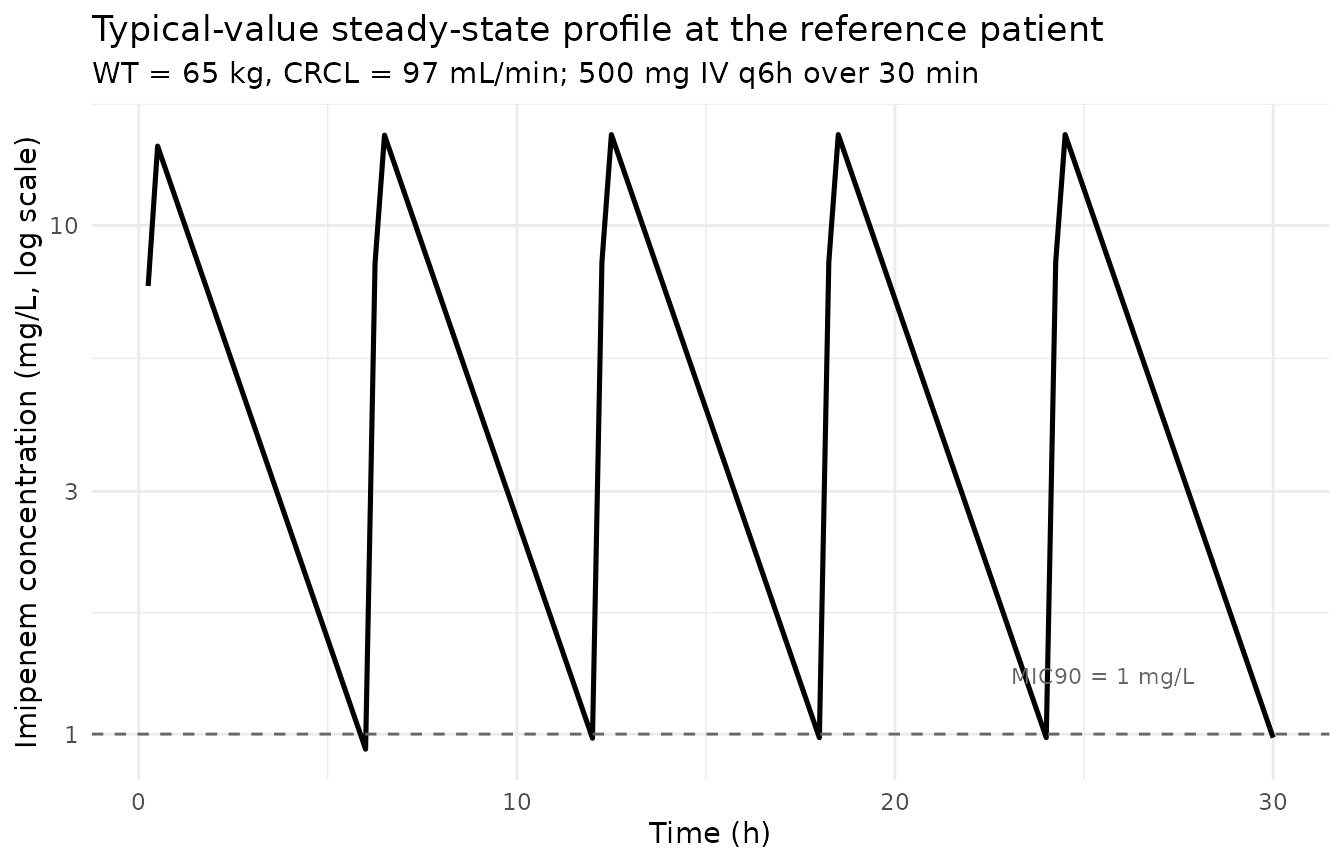
Stochastic VPC across the simulated cohort
sim_stoch |>
  filter(time > 0) |>
  group_by(time) |>
  summarise(
    Q05 = quantile(Cc, 0.05, na.rm = TRUE),
    Q50 = quantile(Cc, 0.50, na.rm = TRUE),
    Q95 = quantile(Cc, 0.95, na.rm = TRUE),
    .groups = "drop"
  ) |>
  ggplot(aes(time, Q50)) +
  geom_ribbon(aes(ymin = Q05, ymax = Q95),
              fill = "gray70", alpha = 0.6) +
  geom_line(linewidth = 0.9) +
  geom_hline(yintercept = 1, linetype = "dashed", colour = "grey40") +
  scale_y_log10() +
  labs(
    x        = "Time (h)",
    y        = "Imipenem concentration (mg/L, log scale)",
    title    = "Stochastic VPC of simulated steady-state profiles",
    subtitle = paste0("Median (line) and 5-95% prediction interval (ribbon); ",
                      "n = ", n_subjects, " subjects, 500 mg IV q6h over 30 min")
  ) +
  theme_minimal()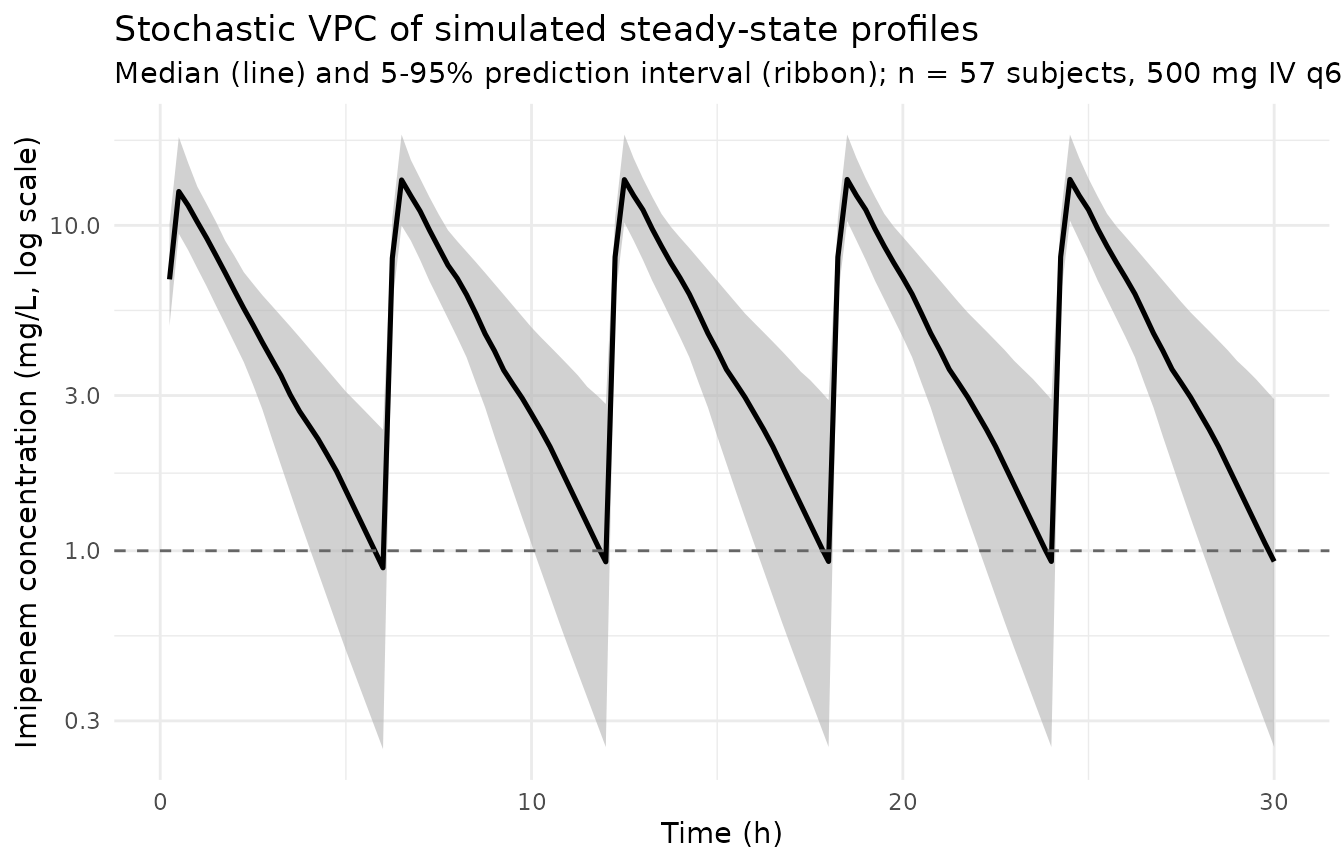
Peak and trough comparison against Table 1
Lamoth 2009 Table 1 reports observed median peak and trough concentrations of 6.6 mg/L (range 0.9-14) and 0.9 mg/L (range 0.25-5) respectively, sampled around a single dose at steady state. Peaks were measured at a median of 2 h after the start of the infusion; troughs 10 minutes before the next dose. The simulated cohort is sampled at the same protocol-matched times below.
peak_window_start  <- max(dose_times) - dose_ii_h + 2 - 0.05
peak_window_end    <- max(dose_times) - dose_ii_h + 2 + 0.05
trough_window_start <- max(dose_times) - 10 / 60 - 0.05
trough_window_end   <- max(dose_times) - 10 / 60 + 0.05

peak_samples <- sim_stoch |>
  filter(time >= peak_window_start, time <= peak_window_end, Cc > 0)
trough_samples <- sim_stoch |>
  filter(time >= trough_window_start, time <= trough_window_end, Cc > 0)

comparison <- tibble::tibble(
  Quantity              = c("Peak (2 h post-dose-start)",
                            "Trough (10 min pre-dose)"),
  `Simulated median`    = c(median(peak_samples$Cc),
                            median(trough_samples$Cc)),
  `Simulated 5-95%`     = c(
    sprintf("%.2f - %.2f",
            quantile(peak_samples$Cc, 0.05),
            quantile(peak_samples$Cc, 0.95)),
    sprintf("%.2f - %.2f",
            quantile(trough_samples$Cc, 0.05),
            quantile(trough_samples$Cc, 0.95))
  ),
  `Published median (Lamoth 2009 Table 1)` = c(6.6, 0.9),
  `Published range (Lamoth 2009 Table 1)`  = c("0.9 - 14", "0.25 - 5")
)
knitr::kable(
  comparison,
  digits  = 2,
  caption = paste0("Simulated peak and trough imipenem concentrations vs. ",
                   "Lamoth 2009 Table 1 (steady-state at 500 mg IV q6h over 30 min).")
)| Quantity | Simulated median | Simulated 5-95% | Published median (Lamoth 2009 Table 1) | Published range (Lamoth 2009 Table 1) |
|---|---|---|---|---|
| Peak (2 h post-dose-start) | 6.90 | 4.53 - 9.22 | 6.6 | 0.9 - 14 |
| Trough (10 min pre-dose) | 1.01 | 0.28 - 3.06 | 0.9 | 0.25 - 5 |
The simulated median peak and trough fall within the published observed ranges; the simulated 5-95% spread is comparable to the observed range.
PKNCA on the simulated cohort
PKNCA computes Cmax, Tmax, and AUC over a single steady-state dosing interval (t = 18 h to t = 24 h, the fifth and final dose in the simulated cohort) so that results are comparable to the steady-state Cmax that the paper observed. A CRCL band (low / median / high CRCL tercile, after dropping the lowest tail to avoid PKNCA’s bin-edge artefacts) is used as the grouping variable so per- band NCA can be compared across the renal-function spectrum.
# CRCL terciles for stratification.
crcl_breaks <- quantile(cov_tab$CRCL, c(0, 1/3, 2/3, 1))
cov_tab$crcl_band <- cut(
  cov_tab$CRCL, breaks = crcl_breaks, include.lowest = TRUE,
  labels = c("low CRCL", "median CRCL", "high CRCL")
)

# Focus the NCA on the final dosing interval (steady state).
ss_start <- max(dose_times)
ss_end   <- ss_start + dose_ii_h

sim_for_nca <- sim_stoch |>
  filter(!is.na(Cc), Cc > 0, time >= ss_start, time <= ss_end) |>
  left_join(cov_tab |> select(id, crcl_band), by = "id") |>
  select(id, time, Cc, crcl_band) |>
  as.data.frame()

doses_for_nca <- events |>
  filter(evid == 1L, time >= ss_start - 0.001) |>
  left_join(cov_tab |> select(id, crcl_band), by = "id") |>
  select(id, time, amt, crcl_band) |>
  as.data.frame()

conc_obj <- PKNCA::PKNCAconc(
  data    = sim_for_nca,
  formula = Cc ~ time | crcl_band + id,
  concu   = "mg/L",
  timeu   = "hr"
)
dose_obj <- PKNCA::PKNCAdose(
  data    = doses_for_nca,
  formula = amt ~ time | crcl_band + id,
  doseu   = "mg"
)

intervals <- data.frame(
  start    = ss_start,
  end      = ss_end,
  cmax     = TRUE,
  tmax     = TRUE,
  auclast  = TRUE,
  cmin     = TRUE
)

nca_data <- PKNCA::PKNCAdata(conc_obj, dose_obj, intervals = intervals)
nca_res  <- suppressWarnings(PKNCA::pk.nca(nca_data))

knitr::kable(
  summary(nca_res),
  caption = paste0("Simulated steady-state NCA parameters by CRCL band ",
                   "(PKNCA; 500 mg IV q6h, fifth dose 18-24 h).")
)| Interval Start | Interval End | crcl_band | N | AUClast (hr*mg/L) | Cmax (mg/L) | Cmin (mg/L) | Tmax (hr) |
|---|---|---|---|---|---|---|---|
| 24 | 30 | low CRCL | 19 | 33.6 [22.8] | 13.7 [17.5] | 1.34 [74.6] | 0.500 [0.500, 0.500] |
| 24 | 30 | median CRCL | 19 | 31.5 [18.5] | 14.5 [18.8] | 0.902 [83.5] | 0.500 [0.500, 0.500] |
| 24 | 30 | high CRCL | 19 | 27.1 [21.0] | 13.5 [21.6] | 0.609 [80.8] | 0.500 [0.500, 0.500] |
Assumptions and deviations
-
IIV is applied multiplicatively to total CL (not to either component alone). Lamoth 2009 Table 2 reports a single inter-individual variability magnitude “(17% +/- 6%)” displayed in the row for Nonrenal CL. The Results paragraph above Table 2 states that the simpler covariate-free 1-compartment model had “26% proportional interpatient variability” on total CL, and that introducing GFR as an explanatory factor for CL improved the fit (
Delta OF = -8.8). The natural NONMEM idiom for an additive split-CL covariate model with a single OMEGA on CL isTVCL = THETA(1) + THETA(2) * GFR / 100 CL = TVCL * exp(ETA(1))i.e. ETA is exponential on the total CL after the GFR covariate. The packaged model uses this parameterization (
cl <- (cl_nonren + cl_renal * CRCL / 100) * exp(etalcl)), giving a residual unexplained 17% CV on total CL that is consistent with the paper’s narrative reduction from 26% to 17%. An alternative reading would place ETA only on the non-renal arm (etalcl_nonren); the placement of “(17% +/- 6%)” within the Nonrenal CL row is consistent with that reading too. Without the underlying NONMEM control stream the two parameterizations cannot be distinguished from Table 2 alone; the present choice is the one that best reconciles the narrative variance reduction. CRCL stored under the canonical
CRCLcolumn despite NOT being BSA-normalized. The canonicalCRCLcolumn ininst/references/covariate-columns.mdaccepts raw Cockcroft-Gault creatinine clearance in mL/min (without BSA normalization) when the source paper uses it that way – following theDelattre_2010_amikacin.RandNA_NA_lidocaine.Rprecedents. Lamoth 2009 Methods explicitly cites the Cockcroft-Gault formula derived from age, sex, total body weight, and serum creatinine; the source column “GFR” reports values in raw mL/min, not in mL/min/1.73 m^2. Reference value 100 mL/min for the linear renal-CL slope (exp(lcl_renal) * CRCL / 100); the population median was 105 mL/min per Table 1. Do not compare the magnitude ofexp(lcl_renal) = 4.79 L/hagainst BSA-normalized reference values in other models – the units differ.Linear (exponent = 1) WT scaling on Vc, no IIV on V. Lamoth 2009 Results paragraph 3 states “The definition of V as a multiple of body weight improved the model (Delta OF = -16.4)” and Table 2 reports “V (liters per 70 kg BW) = 33.5”, consistent with
V_i = 33.5 * (WT_i / 70)^1. The exponent is wrapped infixed(1)inini()so the structural-assumption status is visible in the model metadata. Table 2 reports no IIV magnitude alongside V, so noetalvcis included.No IIV on the renal-CL arm. Table 2 reports only one IIV magnitude (the “(17% +/- 6%)” shown in the Nonrenal CL row), so the renal arm is taken as a deterministic linear function of CRCL with no additional between-subject variability.
One-compartment disposition. Lamoth 2009 Results paragraph 3 states “Introducing a second compartment or testing alternative variability models did not result in a significant decrease of the objective function.” The packaged model uses a single central compartment with IV infusion input, matching the paper’s final-model choice.
omega^2 = log(1 + CV^2). Table 2 reports the BSV as CV%; the corresponding log-normal variance was computed viaomega^2 = log(1 + CV^2)– the standard NONMEM back-transformation – and entered as theetalclinitial value.Race / ethnicity not modeled. Lamoth 2009 does not report race composition (single-centre Swiss university hospital cohort) and the analysis did not test race as a covariate.
Sampling protocol. The vignette samples the trough 10 minutes before the next dose and the peak at 2 h after the start of the dose, matching the protocol in Methods. The published observed peak was sampled at a median of 2 h with a range of 0.5-4 h after the start of the infusion; the vignette uses the median time for the comparison table to keep the sampling deterministic across simulated subjects.
Concentration units. The model uses
mg/L(paper convention for imipenem; the bioanalytical HPLC method is calibrated over 0.25-200 mg/L). With dose inmgandvcinL, the ratiocentral / vcdirectly givesmg/L; no scale factor is applied.Free-drug HPLC measurements. Lamoth 2009 Methods reports that the HPLC assay measures free-circulating imipenem (free fraction). The model treats the observed concentrations as the simulation output without an explicit free / total adjustment, consistent with the paper’s parameterization of the structural model directly against the free-circulating measurements.