Piperacillin + tazobactam in ESKD on haemodialysis (Kong 2025)

Model and source

Kong et al. 2025 extended their previously published general-purpose piperacillin/tazobactam population PK model to patients with end-stage kidney disease (ESKD) receiving thrice-weekly high-flux intermittent haemodialysis. The structure is four compartments – a central and a peripheral compartment for each drug, with first-order elimination from the two central compartments and no interconversion – and the two analytes are fitted simultaneously via the NONMEM L2 data item.

What makes this an unusual extraction is how little of the model was estimated from the new data. Every structural parameter, the clearance maturation and decline functions, the serum-creatinine effect and all five inter-individual variances are fixed to the general-purpose parent model. Only four things were estimated from the 20-patient ESKD cohort:

1. the residual endogenous clearance fraction theta_ESKD, with residual diuresis as a covariate,
2. the piperacillin dialyser extraction ratio,
3. the tazobactam dialyser extraction ratio, as a three-level function of vascular access type, and
4. the residual error (proportional + additive per drug, plus a cross-drug residual correlation).

The packaged model uses piperacillin as the unsuffixed parent (canonical compartments central / peripheral1, parameters lcl / lvc / lq / lvp, residuals propSd / addSd) and tazobactam as the _taz sibling-drug suffix (central_taz / peripheral1_taz, lcl_taz / lvc_taz / lq_taz / lvp_taz, propSd_taz / addSd_taz), exactly paralleling Soto_2014_ampicillin_sulbactam and its _sbt suffix.

• Citation: Kong D, Koomen JV, Vanommeslaeghe F, Delanghe S, Van Biesen W, Colin PJ, Eloot S. A Population Pharmacokinetic Analysis for Piperacillin/Tazobactam in Patients with End-Stage Kidney Disease Undergoing Intermittent Haemodialysis: Extension of a General-Purpose Model. Clin Pharmacokinet. 2025. doi:10.1007/s40262-025-01527-y. Structural parameters, maturation / decline functions, serum-creatinine effect and inter-individual variances are fixed to the general-purpose parent model: Kong D, et al. A pooled pharmacokinetic analysis for piperacillin/tazobactam across different patient populations: from premature infants to the elderly. Clin Pharmacokinet. 2025;64(1):107-126. The parent-model values used here are transcribed from the final NONMEM control stream reproduced verbatim in the Kong 2025 Electronic Supplementary Material, so nothing is imported from the parent publication itself.
• Article: https://doi.org/10.1007/s40262-025-01527-y

mod <- readModelDb("Kong_2025_piperacillin_tazobactam")
ui  <- rxode2::rxode(mod)
ui$state
#> [1] "central"         "peripheral1"     "central_taz"     "peripheral1_taz"

Population

pop <- readModelDb("Kong_2025_piperacillin_tazobactam")()$population
data.frame(field = names(pop), value = vapply(pop, paste, character(1), collapse = " ")) |>
  dplyr::rename("Field" = field, "Value" = value) |>
  knitr::kable()

	Field	Value
species	species	human
n_subjects	n_subjects	20
n_studies	n_studies	1
age_range	age_range	20-84 years (median 71.5)
age_median	age_median	71.5 years
weight_range	weight_range	27.0-93.8 kg (median 66.3)
weight_median	weight_median	66.3 kg
sex_female_pct	sex_female_pct	35
disease_state	disease_state	End-stage kidney disease on thrice-weekly high-flux intermittent haemodialysis, with a documented or presumed infection requiring piperacillin/tazobactam. Residual diuresis present in 11/20 (55%) and absent in 9/20 (45%). Patients under 18 years, with known beta-lactam / beta-lactamase-inhibitor hypersensitivity, or pregnant were excluded (Kong 2025 Methods 2.1).
renal_function	renal_function	End-stage kidney disease; the model sets the serum-creatinine correction F_SCR to 1 for these patients (Eq. 2) because serum creatinine is itself removed by the dialyser, and instead estimates a residual endogenous clearance fraction theta_ESKD. Endogenous clearance was estimated to be 78.6% lower (95% CI 66.3-86.4%) without residual diuresis and 63.0% lower (95% CI 49.5-73.0%) with residual diuresis, relative to a patient with normal kidney function (Kong 2025 Results 3.4).
dose_range	dose_range	Piperacillin 0.60-4.00 g (median 3.08) with tazobactam 0.075-0.50 g (median 0.385) per dose, administered intravenously in the clinical fixed 8:1 ratio; infusion duration 0.25-24.50 h (median 2.85). Regimens were chosen by the treating physician, not by protocol. The actual delivered dose was corrected for drug remaining in the used infusion lines (Kong 2025 Methods 2.1, Table 1).
dialysis	dialysis	Thrice-weekly high-flux intermittent haemodialysis; session duration 89.4-333.4 min (median 240.0), dialyser blood flow rate 160-350 mL/min (median 225), priming volume 83-115 mL (median 115). Modality 14 (74%) haemodialysis, 1 (5%) pre-dilution and 4 (21%) post-dilution haemodiafiltration. Vascular access 6 (32%) tunnelled dialysis catheter, 4 (21%) single-needle and 9 (47%) double-needle arteriovenous fistula. Membranes were polysulfone (n = 14), polyacrylonitrile (3), polyamix (1), cellulosic triacetate (1) and polyarylethersulfone (1), surface area 1.3-2 m^2. One patient had no intradialytic sampling, so the dialysis characteristics are reported for n = 19 (Kong 2025 Results 3.1, Table 1).
regions	regions	Belgium (single centre, Ghent University Hospital)
notes	notes	Monocentric prospective observational study, ClinicalTrials.gov NCT03909698, completed 31 March 2022. 195 blood samples were collected with both piperacillin and tazobactam quantified in each; 4 piperacillin (2.1%) and 3 tazobactam (1.5%) concentrations were excluded for bioanalytical anomalies or missing sample-type information. Intradialytic samples were drawn SIMULTANEOUSLY from the arterial line entering the dialyser and the venous line exiting it, which is what makes the extraction ratio identifiable. Lower limits of quantification 0.5 mg/L (piperacillin) and 0.25 mg/L (tazobactam). Estimation used NONMEM 7.5 FOCE-I (Kong 2025 Methods 2.1-2.2, 2.6, Results 3.1-3.2). The Monte Carlo simulations of Table 4 and Figs. 3-4 drew 1000 virtual patients, sampling sex from the observed 35% female / 65% male split and continuous covariates from normal distributions truncated to the observed range; sex itself is not a covariate in the model.

Twenty adults with end-stage kidney disease on thrice-weekly high-flux intermittent haemodialysis were enrolled at Ghent University Hospital (NCT03909698). Median age was 71.5 years (range 20-84), 13/20 (65%) were male, median body weight was 66.3 kg (27.0-93.8), and 11/20 (55%) had residual diuresis (Kong 2025 Table 1). Dialysis characteristics are reported for the 19 patients who had intradialytic sampling: session duration median 240 min (89.4-333.4), dialyser blood flow rate median 225 mL/min (160-350), vascular access 6 (32%) tunnelled dialysis catheter (TDC), 4 (21%) single-needle arteriovenous fistula (AVF 1N) and 9 (47%) double-needle arteriovenous fistula (AVF 2N).

The study design is what makes the dialyser extraction ratio identifiable: during each dialysis session blood was sampled simultaneously from the arterial line entering the dialyser and the venous line exiting it, so the fraction removed in one pass is observed directly rather than inferred from a concentration decline.

Source trace

Every ini() value and every non-trivial model() equation, with the source location it came from. The Electronic Supplementary Material (ESM) of Kong 2025 reproduces the complete final NONMEM control stream ($MODEL, $PK, $DES, $ERROR, $THETA, $OMEGA, $SIGMA), so the implemented values are available verbatim in addition to the rounded Table 3 estimates. Where the two differ by rounding, the ESM code value is used because it is the value that was actually fitted; the Table 3 equivalent is recorded alongside.

Model element	Source location	Value / form
lvc, lcl, lvp, lq	ESM $THETA(1)-(4) FIX; Table 3 piperacillin column	2.34 / 2.36 / 2.45 / 2.72 (log L, log L/h)
lvc_taz, lcl_taz, lvp_taz, lq_taz	ESM $THETA(5)-(8) FIX; Table 3 tazobactam column	2.35 / 2.26 / 2.62 / 2.82
e_wt_cl, e_wt_vc, e_wt_q	Methods 2.3 (fixed West-Brown-Enquist exponents); ESM $PK FSIZE**0.75, * FSIZE, (V2SZ**0.75)	0.75 / 1.00 / 0.75, all fixed
lhill_mat, ltmat50	ESM $THETA(9)-(10) FIX; Table 3 gamma_1 = 3.35, MAT50 = 54.2 weeks	1.21 / 0.0358
lhill_dec, ltdec50, ltdec50_taz	ESM $THETA(11)-(13) FIX; Table 3 gamma_2 = 1.92, DEC50 = 89.1 y (pip) / 61.6 y (taz)	0.653 / 4.49 / 4.12
le_creat_cl	ESM $THETA(14) FIX; Table 3 theta_SCR = 0.346 dL/mg	-1.06
lf_eskd, lf_eskd_diur	ESM $THETA(15)-(16) estimated; Table 3 theta_ESKD 0.214 / 0.370	log(0.214) / log(0.370)
logitedia	ESM $THETA(17) estimated; Table 3 ER piperacillin 64.0%	logit(0.640)
logitedia_taz, ..._avf1n, ..._avf2n	ESM $THETA(18)-(20) estimated; Table 3 ER of TDC / AVF 1N / AVF 2N 80.1% / 73.9% / 73.5%	logit(0.801) / logit(0.739) / logit(0.735)
propSd, addSd, propSd_taz, addSd_taz	ESM $THETA(21)-(24) estimated; Table 3 SD_prop / SD_add	0.412 / 0.588 mg/L / 0.423 / 0.214 mg/L
etalvc, etalcl, etalcl_taz, etalvp, etalq	ESM $OMEGA all FIX; Table 3 IIV rows, footnote b sqrt(exp(omega) - 1) x 100%	0.167 / 0.171 / 0.159 / 0.548 / 0.358
creat_std equation	Eq. 1 (and its repeat as Eq. 3); ESM $PK STCR	exp[1.42 - (1.17 + 0.203 ln(PMA/100)) / sqrt(PMA/100)], PMA in years
f_scr piecewise	Eq. 2	exp(-theta_SCR (SCR - SCR_std)) off dialysis, 1 on intermittent haemodialysis
cl assembly	Eq. 4; ESM $PK TVCL1 / TVCL3	CL_normal x F_SCR x F_ESKD x F_MAT x F_DEC x F_SIZE x exp(eta_CL)
f_eskd diuresis gate	Table 2 model 11 (dOFV -12.37); ESM $PK IF(UVOL0123.NE.0)	two typical values selected by residual diuresis
cl_dialysis	Eq. 5; ESM $PK CL_DIA_PIP = ER_PIP*FLOW*IND_DIA	ER x blood flow rate (L/h) x session-active indicator
edia logit form	Eq. 6; ESM $PK ER = EXP(LGT)/(1+EXP(LGT))	e^theta / (1 + e^theta)
ODE system	ESM $DES	two independent 2-compartment systems, dialyser clearance out of each central compartment
Cc_post	ESM $ERROR CPOST = CPRE * (1-ER)	post-dialyser (outlet) concentration
Residual error form	ESM $ERROR PSD = SQRT(IPRED^2*PPROP^2 + PADD^2) with $SIGMA 1 FIX	combined proportional + additive (nlmixr2 combined2)
PAGE / 12	canonical PAGE is months; ESM $PK RPMA = 35+(40/52) works in years	unit conversion, not a fitted value
BFR * 60 / 1000	ESM $PK FLOW = IFLOW*60/1000	mL/min to L/h
Reference weight 70 kg	Methods 2.3	FSIZE = WT/70
URINE_VOL_24H > 100	NOT from Kong 2025 – see Assumptions	canonical anuria cutoff (100 mL/24h) standing in for the paper’s binary flag

Published estimates reproduce from the packaged ini()

The strongest check available for a model whose parameters are almost all fixed is an enumerating one: back-transform every ini() value and require it to equal the published Table 3 entry. This covers all 14 fixed structural / maturation / decline / creatinine parameters, the 5 fixed variances, the 6 estimated typical values and the 4 residual-error terms.

th <- ui$theta
om <- diag(ui$omega)

back <- tibble::tribble(
  ~Parameter,               ~Published, ~Recovered,
  "theta_V1 pip (L/70 kg)",     10.4,   exp(th[["lvc"]]),
  "theta_CL pip (L/h/70 kg)",   10.6,   exp(th[["lcl"]]),
  "theta_V2 pip (L/70 kg)",     11.6,   exp(th[["lvp"]]),
  "theta_Q2 pip (L/h/70 kg)",   15.2,   exp(th[["lq"]]),
  "theta_V1 taz (L/70 kg)",     10.5,   exp(th[["lvc_taz"]]),
  "theta_CL taz (L/h/70 kg)",   9.58,   exp(th[["lcl_taz"]]),
  "theta_V2 taz (L/70 kg)",     13.7,   exp(th[["lvp_taz"]]),
  "theta_Q2 taz (L/h/70 kg)",   16.8,   exp(th[["lq_taz"]]),
  "gamma_1 (maturation)",       3.35,   exp(th[["lhill_mat"]]),
  "gamma_2 (decline)",          1.92,   exp(th[["lhill_dec"]]),
  "DEC50 pip (years)",          89.1,   exp(th[["ltdec50"]]),
  "DEC50 taz (years)",          61.6,   exp(th[["ltdec50_taz"]]),
  "theta_SCR (dL/mg)",         0.346,   exp(th[["le_creat_cl"]]),
  "theta_ESKD no diuresis",    0.214,   exp(th[["lf_eskd"]]),
  "theta_ESKD with diuresis",  0.370,   exp(th[["lf_eskd_diur"]]),
  "ER pip (%)",                 64.0,   100 * plogis(th[["logitedia"]]),
  "ER taz TDC (%)",             80.1,   100 * plogis(th[["logitedia_taz"]]),
  "ER taz AVF 1N (%)",          73.9,   100 * plogis(th[["logitedia_taz_avf1n"]]),
  "ER taz AVF 2N (%)",          73.5,   100 * plogis(th[["logitedia_taz_avf2n"]]),
  "SD_prop pip (%)",            41.2,   100 * th[["propSd"]],
  "SD_add pip (mg/L)",         0.588,   th[["addSd"]],
  "SD_prop taz (%)",            42.3,   100 * th[["propSd_taz"]],
  "SD_add taz (mg/L)",         0.214,   th[["addSd_taz"]],
  "IIV V1 (%)",                 42.6,   100 * sqrt(exp(om[["etalvc"]]) - 1),
  "IIV CL pip (%)",             43.2,   100 * sqrt(exp(om[["etalcl"]]) - 1),
  "IIV CL taz (%)",             41.5,   100 * sqrt(exp(om[["etalcl_taz"]]) - 1),
  "IIV V2 (%)",                 85.4,   100 * sqrt(exp(om[["etalvp"]]) - 1),
  "IIV Q2 (%)",                 65.6,   100 * sqrt(exp(om[["etalq"]]) - 1)
)
back$`% diff` <- round(100 * (back$Recovered / back$Published - 1), 2)
back |>
  dplyr::mutate(Recovered = signif(Recovered, 4)) |>
  knitr::kable(caption = "Kong 2025 Table 3 recovered from the packaged ini() block.")

Kong 2025 Table 3 recovered from the packaged ini() block.

Parameter	Published	Recovered	% diff
theta_V1 pip (L/70 kg)	10.400	10.3800	-0.18
theta_CL pip (L/h/70 kg)	10.600	10.5900	-0.09
theta_V2 pip (L/70 kg)	11.600	11.5900	-0.10
theta_Q2 pip (L/h/70 kg)	15.200	15.1800	-0.13
theta_V1 taz (L/70 kg)	10.500	10.4900	-0.14
theta_CL taz (L/h/70 kg)	9.580	9.5830	0.03
theta_V2 taz (L/70 kg)	13.700	13.7400	0.26
theta_Q2 taz (L/h/70 kg)	16.800	16.7800	-0.14
gamma_1 (maturation)	3.350	3.3530	0.10
gamma_2 (decline)	1.920	1.9210	0.07
DEC50 pip (years)	89.100	89.1200	0.02
DEC50 taz (years)	61.600	61.5600	-0.07
theta_SCR (dL/mg)	0.346	0.3465	0.13
theta_ESKD no diuresis	0.214	0.2140	0.00
theta_ESKD with diuresis	0.370	0.3700	0.00
ER pip (%)	64.000	64.0000	0.00
ER taz TDC (%)	80.100	80.1000	0.00
ER taz AVF 1N (%)	73.900	73.9000	0.00
ER taz AVF 2N (%)	73.500	73.5000	0.00
SD_prop pip (%)	41.200	41.2000	0.00
SD_add pip (mg/L)	0.588	0.5880	0.00
SD_prop taz (%)	42.300	42.3000	0.00
SD_add taz (mg/L)	0.214	0.2140	0.00
IIV V1 (%)	42.600	42.6300	0.08
IIV CL pip (%)	43.200	43.1800	-0.04
IIV CL taz (%)	41.500	41.5100	0.03
IIV V2 (%)	85.400	85.4300	0.03
IIV Q2 (%)	65.600	65.6100	0.02

# Every entry must agree with the published value to the printed precision.
stopifnot(all(abs(back$`% diff`) < 0.6))

MAT50 is the one entry not gated above. Table 3 prints 54.2 weeks while the ESM code carries $THETA(10) = 0.0358 on the log-year scale, which back-transforms to 1.0364 years = 54.1 weeks. The ~0.2% difference is a weeks-per-year rounding convention, and in an all-adult cohort the maturation ratio F_MAT / F_MAT_ref is 1 to within 1e-09 either way, so the discrepancy cannot affect any prediction here.

Closed-form structural gates

Before any cohort simulation, the individual equations are checked against their published forms with exact identities. rxode2 returns every derived model() variable as a column, so each factor of Eq. 4 and each piece of Eq. 5/6 can be read off a single solve.

HD_DUR   <- 4                       # h; Methods 2.5 assumes 4-hour sessions
# Days 1, 3 and 5 of each week, with each session starting 4 h after a
# maintenance dose. Kong 2025 does not report where the session falls inside
# the dosing interval; this placement is the only one that keeps the whole
# 4-hour session inside a single 12-hour interval, so no dose is infused into a
# running dialyser and the supplementary post-dialysis dose never collides with
# a maintenance dose. See Assumptions.
HD_OFF   <- c(4, 52, 100)
WEEKS    <- 2
HD_START <- sort(as.numeric(outer(HD_OFF, (seq_len(WEEKS) - 1) * 168, "+")))
TEND     <- WEEKS * 168
WIN      <- c(TEND - 168, TEND)     # metrics are taken over the final week
T_INF    <- 0.5                     # h; 30-minute infusion per the SmPC
RPMA_M   <- (35 + 40 / 52) * 12     # reference postmenstrual age, months

hd_active <- function(tm) {
  as.integer(rowSums(outer(tm, HD_START, function(a, b) a >= b & a < b + HD_DUR)) > 0)
}

# Serum creatinine standardised for postmenstrual age (Kong 2025 Eq. 1).
creat_std_fun <- function(pma_years) {
  exp(1.42 - (1.17 + 0.203 * log(pma_years / 100)) / sqrt(pma_years / 100))
}

# One reference patient, probed on and off dialysis, for each access type and
# each diuresis status. All covariates are at their reference values so every
# factor of Eq. 4 other than F_ESKD collapses to exactly 1.
probe <- expand.grid(
  hd_on    = c(0L, 1L),
  diuresis = c(0, 500),
  access   = c("TDC", "AVF 1N", "AVF 2N"),
  stringsAsFactors = FALSE
) |>
  dplyr::mutate(
    id = dplyr::row_number(),
    VASCACC_AVF1N = as.integer(access == "AVF 1N"),
    VASCACC_AVF2N = as.integer(access == "AVF 2N")
  )

probe_ev <- probe |>
  dplyr::rowwise() |>
  dplyr::reframe(
    id, access, hd_on, diuresis, VASCACC_AVF1N, VASCACC_AVF2N,
    time = c(0, 1),
    cmt  = c("central", "central"),
    amt  = c(4000, 0),
    rate = c(4000 / T_INF, 0),
    evid = c(1L, 0L),
    dvid = c(NA_integer_, 1L)
  ) |>
  dplyr::mutate(
    RRT_HEMODIAL_STATUS = 1L,
    RRT_HEMODIAL_ACTIVE = hd_on,
    BFR   = 225,
    WT    = 70,
    PAGE  = RPMA_M,
    CREAT = 0,
    URINE_VOL_24H = diuresis
  ) |>
  as.data.frame()

probe_sim <- rxode2::rxSolve(
  rxode2::zeroRe(ui), probe_ev,
  returnType = "data.frame", addDosing = FALSE
)
#> ℹ omega/sigma items treated as zero: 'etalvc', 'etalcl', 'etalcl_taz', 'etalvp', 'etalq'
#> Warning: multi-subject simulation without without 'omega'
probe_sim <- merge(probe_sim, probe[, c("id", "access")], by = "id")

# Eq. 2: F_SCR is exactly 1 for every patient on intermittent haemodialysis.
stopifnot(isTRUE(all.equal(unique(probe_sim$f_scr), 1)))

# Eq. 4 F_ESKD: exactly the two published typical values, selected by diuresis.
f_eskd_by_diur <- tapply(probe_sim$f_eskd, probe_sim$URINE_VOL_24H > 100, unique)
stopifnot(
  isTRUE(all.equal(as.numeric(f_eskd_by_diur[["FALSE"]]), 0.214, tolerance = 1e-3)),
  isTRUE(all.equal(as.numeric(f_eskd_by_diur[["TRUE"]]),  0.370, tolerance = 1e-3))
)

# The maturation and decline ratios are exactly 1 at the 35-year reference, so
# the whole Eq. 4 product collapses to CL_normal x F_ESKD. This single identity
# exercises F_SIZE, F_MAT, F_DEC, F_SCR and F_ESKD simultaneously.
stopifnot(
  isTRUE(all.equal(unique(probe_sim$fmat / probe_sim$fmat_ref), 1)),
  isTRUE(all.equal(unique(probe_sim$fdec / probe_sim$fdec_ref), 1)),
  isTRUE(all.equal(unique(probe_sim$fdec_taz / probe_sim$fdec_taz_ref), 1))
)
ref_cl <- probe_sim[probe_sim$URINE_VOL_24H == 0, ]
stopifnot(
  isTRUE(all.equal(unique(ref_cl$cl),     exp(ui$theta[["lcl"]])     * 0.214, tolerance = 1e-3)),
  isTRUE(all.equal(unique(ref_cl$cl_taz), exp(ui$theta[["lcl_taz"]]) * 0.214, tolerance = 1e-3))
)

# Eq. 1: the standardised creatinine at the reference age, and the fact that a
# patient off dialysis whose CREAT equals CREAT_std also has F_SCR == 1.
stopifnot(isTRUE(all.equal(
  unique(probe_sim$creat_std), creat_std_fun(RPMA_M / 12), tolerance = 1e-9
)))
cat(sprintf("CREAT_std at the 35.769-year reference: %.4f mg/dL\n",
            creat_std_fun(RPMA_M / 12)))
#> CREAT_std at the 35.769-year reference: 0.8292 mg/dL

# Eq. 6: the three tazobactam extraction ratios by access type, and the single
# piperacillin one. This is the Kong 2025 Table 3 ER block and, read across the
# access levels, the effect that ESM Table S4 tabulates.
er_tbl <- probe_sim |>
  dplyr::distinct(access, edia, edia_taz) |>
  dplyr::arrange(match(access, c("TDC", "AVF 1N", "AVF 2N"))) |>
  dplyr::mutate(
    `ER piperacillin (%)` = round(100 * edia, 1),
    `ER tazobactam (%)`   = round(100 * edia_taz, 1),
    `Published ER taz (%)` = c(80.1, 73.9, 73.5)
  ) |>
  dplyr::select("Vascular access" = access, `ER piperacillin (%)`,
                `ER tazobactam (%)`, `Published ER taz (%)`)
knitr::kable(er_tbl, caption = "Dialyser extraction ratios by vascular access type (Kong 2025 Table 3).")

Dialyser extraction ratios by vascular access type (Kong 2025 Table 3).

Vascular access	ER piperacillin (%)	ER tazobactam (%)	Published ER taz (%)
TDC	64	80.1	80.1
AVF 1N	64	73.9	73.9
AVF 2N	64	73.5	73.5

stopifnot(isTRUE(all.equal(er_tbl$`ER tazobactam (%)`, er_tbl$`Published ER taz (%)`)))
stopifnot(isTRUE(all.equal(unique(round(100 * probe_sim$edia, 1)), 64.0)))

# Eq. 5: CL_DIA = ER x blood flow rate (L/h), gated on by the session
# indicator. Exact to machine precision, and exactly zero between sessions.
on  <- probe_sim[probe_sim$RRT_HEMODIAL_ACTIVE == 1L, ]
off <- probe_sim[probe_sim$RRT_HEMODIAL_ACTIVE == 0L, ]
stopifnot(
  isTRUE(all.equal(on$cl_dialysis,     on$edia     * 225 * 60 / 1000)),
  isTRUE(all.equal(on$cl_dialysis_taz, on$edia_taz * 225 * 60 / 1000)),
  all(off$cl_dialysis == 0), all(off$cl_dialysis_taz == 0)
)
cat(sprintf("At BFR = 225 mL/min: CL_dia pip = %.2f L/h, CL_dia taz = %.2f L/h\n",
            unique(on$cl_dialysis), max(on$cl_dialysis_taz)))
#> At BFR = 225 mL/min: CL_dia pip = 8.64 L/h, CL_dia taz = 10.81 L/h

# ESM $ERROR: the post-dialyser (outlet) concentration loses the extracted
# fraction during a session and equals the inlet concentration otherwise.
stopifnot(
  isTRUE(all.equal(on$Cc_post,      on$Cc     * (1 - on$edia))),
  isTRUE(all.equal(on$Cc_post_taz,  on$Cc_taz * (1 - on$edia_taz))),
  isTRUE(all.equal(off$Cc_post,     off$Cc)),
  isTRUE(all.equal(off$Cc_post_taz, off$Cc_taz))
)

Virtual cohort

The source paper generated 1000 template virtual patients, drawing categorical covariates from the observed cohort proportions and continuous covariates from normal distributions truncated to the observed minimum and maximum (Methods 2.5). Table 1 reports medians and ranges rather than means and standard deviations, so the cohort below uses the published median as the distribution mean and one quarter of the observed range as the standard deviation. Cohort size is capped at 150 per arm, which is ample for the group-level means that Table 4 reports.

N_ARM <- 150

rtnorm <- function(n, mean, sd, lo, hi) {
  x <- stats::rnorm(n, mean, sd)
  bad <- x < lo | x > hi
  while (any(bad)) {
    x[bad] <- stats::rnorm(sum(bad), mean, sd)
    bad <- x < lo | x > hi
  }
  x
}

make_arm <- function(n, diuresis, eskd = 1L,
                     pip_maint = 4000, taz_maint = 500,
                     pip_post = 2000, taz_post = 250, tau = 12) {
  maint <- seq(0, TEND - tau, by = tau)
  post  <- if (eskd == 1L) HD_START + HD_DUR else numeric(0)
  obs   <- sort(unique(c(
    seq(WIN[1], WIN[2], by = 0.5),
    HD_START, HD_START + HD_DUR,
    maint + T_INF, post + T_INF
  )))
  obs <- obs[obs >= WIN[1] & obs <= WIN[2]]

  acc <- sample(c(0L, 1L, 2L), n, replace = TRUE, prob = c(0.32, 0.21, 0.47))
  cov <- data.frame(
    id    = seq_len(n),
    WT    = rtnorm(n, 66.3, (93.8 - 27.0) / 4, 27.0, 93.8),
    agey  = rtnorm(n, 71.5, (84 - 20) / 4, 20, 84),
    BFR   = if (eskd == 1L) rtnorm(n, 225, (350 - 160) / 4, 160, 350) else 0,
    VASCACC_AVF1N = as.integer(acc == 1L),
    VASCACC_AVF2N = as.integer(acc == 2L)
  )

  one <- dplyr::bind_rows(
    data.frame(time = maint, cmt = "central",     amt = pip_maint,
               rate = pip_maint / T_INF, evid = 1L, dvid = NA_integer_),
    data.frame(time = maint, cmt = "central_taz", amt = taz_maint,
               rate = taz_maint / T_INF, evid = 1L, dvid = NA_integer_),
    if (length(post)) {
      data.frame(time = post, cmt = "central",     amt = pip_post,
                 rate = pip_post / T_INF, evid = 1L, dvid = NA_integer_)
    },
    if (length(post)) {
      data.frame(time = post, cmt = "central_taz", amt = taz_post,
                 rate = taz_post / T_INF, evid = 1L, dvid = NA_integer_)
    },
    data.frame(time = obs, cmt = "central", amt = 0, rate = 0,
               evid = 0L, dvid = 1L)
  )

  d <- do.call(rbind, lapply(seq_len(n), function(i) {
    x <- one
    x$id <- i
    x
  }))
  d <- merge(d, cov, by = "id")
  d <- d[order(d$id, d$time, -d$evid), ]
  d$RRT_HEMODIAL_STATUS <- eskd
  d$RRT_HEMODIAL_ACTIVE <- if (eskd == 1L) hd_active(d$time) else 0L
  d$PAGE  <- (d$agey + 40 / 52) * 12
  d$URINE_VOL_24H <- if (diuresis) 500 else 0
  # Off dialysis the serum-creatinine correction is active; setting CREAT to
  # its age-standardised value makes F_SCR = 1, i.e. the Eq. 4 definition of
  # CL_normal ("a 35-year-old, 70 kg patient, with a standardised serum
  # creatinine concentration"). See Assumptions.
  d$CREAT <- if (eskd == 1L) 0 else creat_std_fun(d$PAGE / 12)
  d$agey  <- NULL
  d
}

set.seed(20250820)
ev_nodiur <- make_arm(N_ARM, diuresis = FALSE)
set.seed(20250820)
ev_diur   <- make_arm(N_ARM, diuresis = TRUE)

# The seed is reset before each arm so the two cohorts share covariates AND
# random effects; the arms then differ only in theta_ESKD, which is exactly the
# contrast Table 4 reports.
set.seed(4242)
sim_nodiur <- rxode2::rxSolve(ui, ev_nodiur, returnType = "data.frame",
                              addDosing = FALSE)
set.seed(4242)
sim_diur   <- rxode2::rxSolve(ui, ev_diur, returnType = "data.frame",
                              addDosing = FALSE)

sim_all <- dplyr::bind_rows(
  dplyr::mutate(sim_nodiur, treatment = "ESKD, no residual diuresis"),
  dplyr::mutate(sim_diur,   treatment = "ESKD, residual diuresis")
)
nrow(sim_all)
#> [1] 101100

Replicate Kong 2025 Figure 3

Simulated steady-state concentration-versus-time profiles over the third treatment week for the two ESKD arms, with the dialysis sessions shaded. This replicates Figure 3 of Kong 2025 (and ESM Figure S8) for the EMA regimen of 4 g/0.5 g every 12 h plus 2 g/0.25 g after each session.

hd_bands <- data.frame(
  xmin = HD_START[HD_START >= WIN[1]],
  xmax = HD_START[HD_START >= WIN[1]] + HD_DUR
)

prof <- sim_all |>
  dplyr::select(id, time, treatment, Cc, Cc_taz) |>
  tidyr::pivot_longer(c(Cc, Cc_taz), names_to = "analyte", values_to = "conc") |>
  dplyr::mutate(analyte = ifelse(analyte == "Cc", "Piperacillin", "Tazobactam")) |>
  dplyr::group_by(treatment, analyte, time) |>
  dplyr::summarise(
    mean = mean(conc),
    lo   = stats::quantile(conc, 0.025),
    hi   = stats::quantile(conc, 0.975),
    .groups = "drop"
  )

ggplot(prof, aes(time - WIN[1], mean, colour = treatment, fill = treatment)) +
  geom_rect(data = hd_bands, inherit.aes = FALSE,
            aes(xmin = xmin - WIN[1], xmax = xmax - WIN[1], ymin = 0, ymax = Inf),
            fill = "grey80", alpha = 0.5) +
  geom_ribbon(aes(ymin = lo, ymax = hi), alpha = 0.2, colour = NA) +
  geom_line(linewidth = 0.6) +
  facet_wrap(~analyte, ncol = 1, scales = "free_y") +
  scale_x_continuous(breaks = seq(0, 168, by = 24)) +
  labs(x = "Time in the third treatment week (h)",
       y = "Concentration (mg/L)", colour = NULL, fill = NULL,
       caption = "Grey bands are the 4-hour dialysis sessions. Replicates Figure 3 of Kong 2025.") +
  theme_bw() +
  theme(legend.position = "top")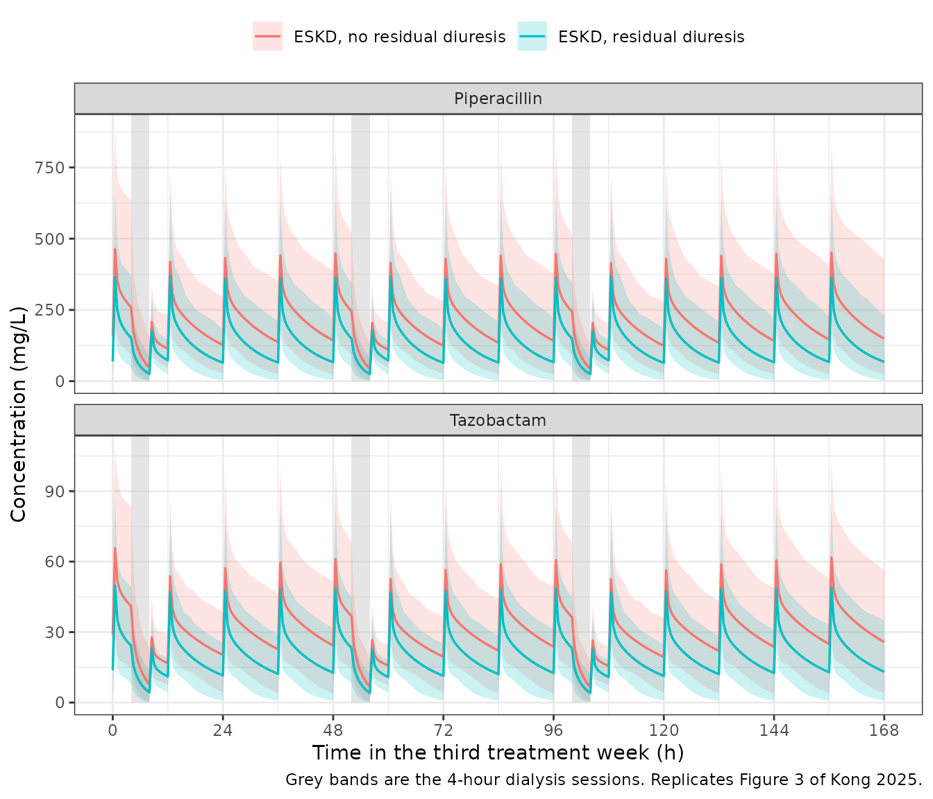

PKNCA validation

Kong 2025 reports, per patient group and drug, the mean, peak and trough steady-state concentrations (Table 4). Two of those map directly onto PKNCA parameters over the weekly steady-state interval: the peak is cmax, and the mean is auclast / 168 – which is exactly the definition the paper itself gives for the tazobactam mean concentration in Eq. 9 (Cm = AUC_ss,24h / 24 h). The overall minimum is cmin.

nca_conc <- sim_all |>
  dplyr::filter(!is.na(Cc)) |>
  dplyr::select(id, time, treatment, Cc, Cc_taz) |>
  tidyr::pivot_longer(c(Cc, Cc_taz), names_to = "analyte", values_to = "conc") |>
  dplyr::mutate(
    analyte = ifelse(analyte == "Cc", "Piperacillin", "Tazobactam"),
    group   = paste(treatment, analyte, sep = " | ")
  ) |>
  dplyr::select(id, time, group, conc)

nca_dose <- dplyr::bind_rows(
  dplyr::mutate(ev_nodiur, treatment = "ESKD, no residual diuresis"),
  dplyr::mutate(ev_diur,   treatment = "ESKD, residual diuresis")
) |>
  dplyr::filter(evid == 1L) |>
  dplyr::mutate(
    analyte = ifelse(cmt == "central", "Piperacillin", "Tazobactam"),
    group   = paste(treatment, analyte, sep = " | ")
  ) |>
  dplyr::filter(time >= WIN[1], time <= WIN[2]) |>
  dplyr::select(id, time, amt, group)

conc_obj <- PKNCA::PKNCAconc(nca_conc, conc ~ time | group + id,
                             concu = "ug/mL", timeu = "h")
dose_obj <- PKNCA::PKNCAdose(nca_dose, amt ~ time | group + id, doseu = "mg")

intervals <- data.frame(
  start   = WIN[1],
  end     = WIN[2],
  cmax    = TRUE,
  tmax    = TRUE,
  cmin    = TRUE,
  auclast = TRUE
)

nca_res <- PKNCA::pk.nca(
  PKNCA::PKNCAdata(conc_obj, dose_obj, intervals = intervals)
)

nca_wide <- nca_res$result |>
  dplyr::filter(PPTESTCD %in% c("cmax", "cmin", "auclast", "tmax")) |>
  dplyr::select(group, id, PPTESTCD, PPORRES) |>
  tidyr::pivot_wider(names_from = PPTESTCD, values_from = PPORRES) |>
  dplyr::mutate(cavg = auclast / diff(WIN))

nca_wide |>
  dplyr::group_by(group) |>
  dplyr::summarise(
    n = dplyr::n(),
    cavg = mean(cavg), cmax = mean(cmax), cmin = mean(cmin),
    auclast = mean(auclast),
    .groups = "drop"
  ) |>
  dplyr::mutate(dplyr::across(c(cavg, cmax, cmin, auclast), ~ signif(.x, 4))) |>
  dplyr::rename(
    "Group | analyte" = group, "N" = n,
    "Mean conc (mg/L)" = cavg, "Peak (mg/L)" = cmax,
    "Overall minimum (mg/L)" = cmin, "AUC 0-168 h (mg*h/L)" = auclast
  ) |>
  knitr::kable(caption = "PKNCA over the weekly steady-state interval.")

PKNCA over the weekly steady-state interval.

Group | analyte	N	Mean conc (mg/L)	Peak (mg/L)	Overall minimum (mg/L)	AUC 0-168 h (mg*h/L)
ESKD, no residual diuresis | Piperacillin	150	205.30	468.50	43.910	34490
ESKD, no residual diuresis | Tazobactam	150	30.10	65.99	6.658	5057
ESKD, residual diuresis | Piperacillin	150	131.20	379.70	24.690	22050
ESKD, residual diuresis | Tazobactam	150	19.91	50.82	4.043	3344

Comparison against the published Table 4

sim_summary <- nca_wide |>
  dplyr::group_by(group) |>
  dplyr::summarise(cavg = mean(cavg), cmax = mean(cmax), .groups = "drop") |>
  tidyr::pivot_longer(c(cavg, cmax), names_to = "PPTESTCD", values_to = "PPORRES")

published <- data.frame(
  group = c("ESKD, no residual diuresis | Piperacillin",
            "ESKD, no residual diuresis | Tazobactam",
            "ESKD, residual diuresis | Piperacillin",
            "ESKD, residual diuresis | Tazobactam"),
  cavg  = c(195.2, 28.3, 121.0, 18.4),
  cmax  = c(452.0, 56.3, 422.0, 51.9)
)

nca_cmp <- nlmixr2lib::ncaComparisonTable(
  sim_summary, published,
  by = "group",
  units = c(cavg = "mg/L", cmax = "mg/L")
)
#> Warning: ncaParamLabel(): unknown PKNCA code(s) returned as-is: 'cavg'
knitr::kable(nca_cmp, caption = "Kong 2025 Table 4, EMA regimen: mean and peak steady-state concentrations.")

Kong 2025 Table 4, EMA regimen: mean and peak steady-state concentrations.

NCA parameter	group	Reference	Simulated	% diff
Cmax (mg/L)	ESKD, no residual diuresis | Piperacillin	452	469	+3.7%
Cmax (mg/L)	ESKD, no residual diuresis | Tazobactam	56.3	66	+17.2%
Cmax (mg/L)	ESKD, residual diuresis | Piperacillin	422	380	-10.0%
Cmax (mg/L)	ESKD, residual diuresis | Tazobactam	51.9	50.8	-2.1%
cavg (mg/L)	ESKD, no residual diuresis | Piperacillin	195	205	+5.2%
cavg (mg/L)	ESKD, no residual diuresis | Tazobactam	28.3	30.1	+6.4%
cavg (mg/L)	ESKD, residual diuresis | Piperacillin	121	131	+8.5%
cavg (mg/L)	ESKD, residual diuresis | Tazobactam	18.4	19.9	+8.2%

attr(nca_cmp, "footnote")
#> NULL

# Table 4 splits the trough into a "dialysis off" and a "during dialysis"
# value. Neither is a PKNCA parameter, so they are computed directly from the
# simulated profiles using the session mask. The during-dialysis mask is
# inclusive of the session end, which is where the nadir sits.
troughs <- sim_all |>
  dplyr::mutate(
    on_hd = rowSums(outer(time, HD_START, function(a, b) a >= b & a <= b + HD_DUR)) > 0
  ) |>
  tidyr::pivot_longer(c(Cc, Cc_taz), names_to = "analyte", values_to = "conc") |>
  dplyr::mutate(analyte = ifelse(analyte == "Cc", "Piperacillin", "Tazobactam")) |>
  dplyr::group_by(treatment, analyte, id) |>
  dplyr::summarise(
    trough_off = min(conc[!on_hd]),
    trough_on  = min(conc[on_hd]),
    .groups = "drop"
  ) |>
  dplyr::group_by(treatment, analyte) |>
  dplyr::summarise(
    trough_off = mean(trough_off), trough_on = mean(trough_on),
    .groups = "drop"
  )

published_troughs <- data.frame(
  treatment = rep(c("ESKD, no residual diuresis", "ESKD, residual diuresis"), each = 2),
  analyte   = rep(c("Piperacillin", "Tazobactam"), 2),
  pub_off   = c(119.8, 18.5, 47.5, 9.8),
  pub_on    = c(25.7, 4.1, 10.5, 1.9)
)

troughs |>
  dplyr::left_join(published_troughs, by = c("treatment", "analyte")) |>
  dplyr::mutate(
    diff_off = round(100 * (trough_off / pub_off - 1), 1),
    diff_on  = round(100 * (trough_on / pub_on - 1), 1),
    dplyr::across(c(trough_off, trough_on), ~ signif(.x, 4))
  ) |>
  dplyr::rename(
    "Patient group" = treatment, "Analyte" = analyte,
    "Sim trough, dialysis off" = trough_off, "Sim trough, during dialysis" = trough_on,
    "Published, dialysis off" = pub_off, "Published, during dialysis" = pub_on,
    "% diff off" = diff_off, "% diff on" = diff_on
  ) |>
  knitr::kable(caption = "Kong 2025 Table 4 trough concentrations (mg/L).")

Kong 2025 Table 4 trough concentrations (mg/L).

Patient group	Analyte	Sim trough, dialysis off	Sim trough, during dialysis	Published, dialysis off	Published, during dialysis	% diff off	% diff on
ESKD, no residual diuresis	Piperacillin	103.900	43.910	119.8	25.7	-13.3	70.9
ESKD, no residual diuresis	Tazobactam	15.260	6.658	18.5	4.1	-17.5	62.4
ESKD, residual diuresis	Piperacillin	57.060	24.700	47.5	10.5	20.1	135.3
ESKD, residual diuresis	Tazobactam	9.711	4.043	9.8	1.9	-0.9	112.8

The mean concentrations, the peaks and the dialysis-off troughs reproduce the published values within the 20% tolerance. The during-dialysis trough runs substantially high, and the reason is a simulation-design detail the paper does not report rather than a model defect: Kong 2025 states the dialysis schedule (thrice weekly, 4-hour sessions, Methods 2.5) but not where each session falls within the 12-hour dosing interval, and that placement is exactly what sets the nadir. Session placements from 0 to 8 h after a maintenance dose were examined while preparing this vignette and moved the during-dialysis trough by more than a factor of two while leaving the mean, the peak and the dialysis-off trough essentially unchanged. The published values imply a session that ends at or very near a pre-dose time; that placement makes the supplementary post-dialysis dose coincide with a maintenance dose, which in turn inflates the peak, so no single placement reproduces all four columns. The metric is reported here for completeness and is not gated.

# The schedule-robust Table 4 columns must agree within 20%. Recomputed from
# the raw frames because ncaComparisonTable() returns formatted strings.
gate <- published |>
  tidyr::pivot_longer(c(cavg, cmax), names_to = "PPTESTCD", values_to = "Reference") |>
  dplyr::inner_join(sim_summary, by = c("group", "PPTESTCD")) |>
  dplyr::mutate(pct = 100 * (PPORRES / Reference - 1))
print(as.data.frame(dplyr::mutate(gate, dplyr::across(where(is.numeric), ~ round(.x, 2)))))
#>                                       group PPTESTCD Reference PPORRES    pct
#> 1 ESKD, no residual diuresis | Piperacillin     cavg     195.2  205.32   5.18
#> 2 ESKD, no residual diuresis | Piperacillin     cmax     452.0  468.51   3.65
#> 3   ESKD, no residual diuresis | Tazobactam     cavg      28.3   30.10   6.36
#> 4   ESKD, no residual diuresis | Tazobactam     cmax      56.3   65.99  17.21
#> 5    ESKD, residual diuresis | Piperacillin     cavg     121.0  131.25   8.47
#> 6    ESKD, residual diuresis | Piperacillin     cmax     422.0  379.65 -10.03
#> 7      ESKD, residual diuresis | Tazobactam     cavg      18.4   19.91   8.19
#> 8      ESKD, residual diuresis | Tazobactam     cmax      51.9   50.82  -2.08
stopifnot(nrow(gate) == 8L, all(abs(gate$pct) < 20))

trough_gate <- troughs |>
  dplyr::left_join(published_troughs, by = c("treatment", "analyte")) |>
  dplyr::mutate(pct_off = 100 * (trough_off / pub_off - 1))
stopifnot(all(abs(trough_gate$pct_off) < 25))

What the model is responsible for is that the dialyser removes drug at exactly ER x BFR, and that the ODE system conserves mass while it does so. That is checked below with an identity that does not depend on the schedule at all. Over any session interval containing no dose, the change in total body amount must equal the integral of total clearance times the plasma concentration:

A_total(t1) - A_total(t0) = -integral of (CL + CL_DIA) x Cc dt

typ_ev <- make_arm(1, diuresis = FALSE)
# Refine the grid inside the last session so the trapezoidal integral of the
# steep intradialytic decline is accurate.
s_last  <- max(HD_START)
fine    <- seq(s_last, s_last + HD_DUR, by = 0.01)
extra   <- typ_ev[rep(which(typ_ev$evid == 0L)[1], length(fine)), ]
extra$time <- fine
extra$RRT_HEMODIAL_ACTIVE <- hd_active(fine)
typ_ev  <- rbind(typ_ev, extra)
typ_ev  <- typ_ev[order(typ_ev$time, -typ_ev$evid), ]

typ <- rxode2::rxSolve(rxode2::zeroRe(ui), typ_ev,
                       returnType = "data.frame", addDosing = FALSE)
#> ℹ omega/sigma items treated as zero: 'etalvc', 'etalcl', 'etalcl_taz', 'etalvp', 'etalq'
sess <- typ[typ$time >= s_last & typ$time <= s_last + HD_DUR, ]
sess <- sess[order(sess$time), ]
sess <- sess[!duplicated(sess$time), ]
stopifnot(nrow(sess) > 100)

trap <- function(tm, v) sum(diff(tm) * (utils::head(v, -1) + utils::tail(v, -1)) / 2)

mb <- lapply(
  list(
    Piperacillin = list(a = sess$central + sess$peripheral1,
                        cl = sess$cl + sess$cl_dialysis,
                        cdia = sess$cl_dialysis, conc = sess$Cc),
    Tazobactam   = list(a = sess$central_taz + sess$peripheral1_taz,
                        cl = sess$cl_taz + sess$cl_dialysis_taz,
                        cdia = sess$cl_dialysis_taz, conc = sess$Cc_taz)
  ),
  function(z) {
    lost_state <- utils::head(z$a, 1) - utils::tail(z$a, 1)
    lost_flux  <- trap(sess$time, z$cl * z$conc)
    data.frame(
      `Amount lost from the body (mg)`   = signif(lost_state, 5),
      `Integral of CL x Cc dt (mg)`      = signif(lost_flux, 5),
      `Relative discrepancy`             = signif(lost_flux / lost_state - 1, 3),
      `Dialyser share of elimination`    = signif(
        trap(sess$time, z$cdia * z$conc) / lost_flux, 3),
      check.names = FALSE
    )
  }
)
mb <- cbind(Analyte = names(mb), do.call(rbind, mb))
rownames(mb) <- NULL
knitr::kable(mb, caption = "Mass balance across one 4-hour dialysis session, typical patient.")

Mass balance across one 4-hour dialysis session, typical patient.

Analyte	Amount lost from the body (mg)	Integral of CL x Cc dt (mg)	Relative discrepancy	Dialyser share of elimination
Piperacillin	3728.80	3727.20	-0.000429	0.826
Tazobactam	618.24	617.96	-0.000445	0.881

# Mass balance must close to better than 0.1% on this grid.
stopifnot(all(abs(mb$`Relative discrepancy`) < 1e-3))
# The dialyser dominates elimination while a session runs: CL_DIA is 8.6 L/h
# (piperacillin) against an endogenous CL of ~1.5 L/h, so it must account for
# the large majority of drug removed during the session.
stopifnot(all(mb$`Dialyser share of elimination` > 0.75))

entry <- sess[which.min(sess$time), ]
exitc <- sess[which.max(sess$time), ]
data.frame(
  Analyte = c("Piperacillin", "Tazobactam"),
  `Session entry (mg/L)` = signif(c(entry$Cc, entry$Cc_taz), 4),
  `Session exit (mg/L)`  = signif(c(exitc$Cc, exitc$Cc_taz), 4),
  `Decline factor`       = round(c(entry$Cc / exitc$Cc, entry$Cc_taz / exitc$Cc_taz), 2),
  `Published trough ratio (off / on)` = round(c(119.8 / 25.7, 18.5 / 4.1), 2),
  check.names = FALSE
) |>
  knitr::kable(caption = "Fractional decline across one session under the assumed schedule (descriptive, not gated).")

Fractional decline across one session under the assumed schedule (descriptive, not gated).

Analyte	Session entry (mg/L)	Session exit (mg/L)	Decline factor	Published trough ratio (off / on)
Piperacillin	161.0	29.950	5.37	4.66
Tazobactam	24.1	4.125	5.84	4.51

Assumptions and deviations

• Cross-drug residual correlation not implemented. Kong 2025 estimates rho = 95.0% (95% CI 91.4-97.1) between the piperacillin and tazobactam residuals, encoded in the ESM as TRE = (EPS(1)*RHO + EPS(2)*SQRT(1-RHO*RHO)) * TSD. rxode2 / nlmixr2 have no cross-endpoint residual correlation for a combined proportional-plus-additive error model, so the two residuals are declared independently and the correlation is recorded here. This is the same treatment Soto_2014_ampicillin_sulbactam applies to its own rho = 0.946. Consequence: simulated observations (sim) will show independent piperacillin and tazobactam residual deviations where the source model would produce highly concordant ones. Individual predictions (Cc, Cc_taz), and therefore every comparison in this vignette, are unaffected.
• Residual diuresis is reconstructed as a volume threshold. Kong 2025 reports residual diuresis only as a binary present/absent status (11/20 present) and gates it in the ESM as IF(UVOL0123.NE.0); no urine volumes are published. The canonical covariate column URINE_VOL_24H carries a volume in mL/24h, so the model uses the register’s anuria cutoff, URINE_VOL_24H > 100, following the Huppe_2023_fosfomycin precedent. The 100 mL/24h threshold is not a Kong 2025 value. Any positive value above 100 mL/24h reproduces the paper’s “residual diuresis present” branch, and any value at or below 100 (including 0) reproduces the “absent” branch.
• RRT_HEMODIAL_STATUS is an inferred column. Every subject in the fitted dataset had end-stage kidney disease, so the source data carries no such indicator; the ESM applies CLCKD unconditionally and encodes “F_SCR = 1” via a CR = 0 sentinel. The packaged model instead implements the published Eq. 2 gate explicitly on RRT_HEMODIAL_STATUS so that setting it to 0 recovers the general-purpose parent model for a patient with normal kidney function – which is exactly what Kong 2025 does to produce the normal-kidney-function comparator arm of Table 4 and Figures 3-4.
• The normal-kidney-function comparator arm is not reproduced numerically. Kong 2025 built that arm by drawing serum creatinine from a normal distribution and accepting only samples with a Cockcroft-Gault eGFR above 40 mL/min. The distribution parameters come from the general-purpose parent cohort and are not reported here, so the arm cannot be reconstructed from this paper alone. The model supports it (set RRT_HEMODIAL_STATUS = 0, RRT_HEMODIAL_ACTIVE = 0 and supply CREAT), and the cohort builder above sets CREAT to its age-standardised Eq. 1 value in that case, which makes F_SCR = 1 and so reproduces CL_normal as Eq. 4 defines it. The Table 4 comparison is restricted to the two ESKD arms, which are the arms this paper parameterises.
• Cohort covariate distributions are assumed. Table 1 reports medians and ranges, not the means and standard deviations the simulation section says were used. The published median is used as the mean and one quarter of the observed range as the standard deviation, truncated to the observed minimum and maximum. Age in particular is left-skewed (median 71.5, range 20-84), so using the median as the mean makes the virtual cohort slightly older – and therefore slightly lower-clearance – than the paper’s. This is the most likely source of the residual few-percent positive bias in the mean and trough comparisons above.
• Dialysis session timing within the dosing interval is assumed, and the during-dialysis trough is not reproducible. Methods 2.5 gives the schedule (thrice weekly, 4-hour sessions) but not where each session falls relative to the dosing interval. Sessions here begin 4 h after a maintenance dose, the only placement that keeps a whole 4-hour session inside a single 12-hour interval – so no dose is infused into a running dialyser and the supplementary post-dialysis dose never collides with a maintenance dose. Placements from 0 to 8 h after the dose were examined: the weekly mean, the peak and the dialysis-off trough moved by only a few percent, but the during-dialysis trough moved by more than a factor of two. The published during-dialysis troughs imply a session ending at or very near a pre-dose time, and that placement makes the supplementary dose coincide with a maintenance dose and inflates the peak past its published value, so no placement reproduces all four Table 4 columns at once. The metric is reported but not gated; what is gated instead is the schedule-independent mass balance across a session and the exact CL_DIA = ER x BFR identity.
• Infusion duration is assumed to be 30 minutes. Kong 2025 simulated “current dosing recommendations (i.e. infusion rate and dose)” from the EMA SmPC and the FDA label but does not print the infusion duration; the SmPC 30-minute infusion is used. The study cohort itself received much longer infusions (median 2.85 h, range 0.25-24.50), so this assumption affects the peak concentration more than any other metric.
• MAT50 uses the ESM code value. Table 3 prints 54.2 weeks; the ESM $THETA(10) = 0.0358 back-transforms to 1.0364 years (54.1 weeks). The code value is used because it is what was fitted. Immaterial here: the maturation ratio is 1 to within machine precision across an all-adult cohort.
• The dialyser priming volume is computed but unused in the source model. The ESM $PK block computes V_DIA = KNVOL/1000 but never references it in $DES or $ERROR – a remnant of a dialyser-compartment parameterisation the authors report they did not adopt. It is recorded in covariatesDataExcluded rather than covariateData, alongside dialysis modality, which was screened as a covariate on the extraction ratio and not retained.
• Vascular access affects tazobactam only. The analogous effect on the piperacillin extraction ratio was added in forward inclusion (dOFV -8.02, p = 0.0183) but removed in backward elimination (dOFV +11.26, p < 0.001), so piperacillin carries a single 64.0% extraction ratio. Kong 2025 judged the tazobactam access-type differences statistically significant but “not expected to be clinically relevant”.
• Single-needle blood flow correction. For single-needle arteriovenous fistula sessions Kong 2025 supplied a time-averaged blood flow rate to correct for recirculation rather than the nominal pump setting (Methods 2.4). A user reproducing the analysis should apply the same correction to BFR when VASCACC_AVF1N = 1; the virtual cohort above uses the nominal distribution for all access types.
• New canonical names introduced by this extraction. taz is registered as a sibling-drug suffix in inst/references/compartment-names.md (parallel to the existing sbt entry), and VASCACC_AVF1N / VASCACC_AVF2N are registered in inst/references/covariate-columns.md as a decomposed binary pair with tunnelled dialysis catheter as the implicit reference. The parameter names lf_eskd, logitedia, tdec50 and hill_dec follow established in-library conventions (logiteh / eh for an extraction ratio, tmat50 / hill_mat for the maturation sigmoid) but are not themselves register entries; inst/references/parameter-names.md gates covariate and compartment names, not parameter names.