Epetraborole (Ganesan 2022)

Model and source

• Citation: Ganesan H, Safir MC, Bhavnani SM, Krause KM, Rubino CM. 593. Population Pharmacokinetic Model Development for Epetraborole and Mycobacterium avium Complex (MAC) Lung Disease Patients Using Data from Phase 1 and 2 Studies. Open Forum Infect Dis. 2022;9(Suppl 2):S325-S326. doi:10.1093/ofid/ofac492.645 (IDWeek 2022 poster 593). Parameter estimates: abstract Table 2 (identical in the poster).
• Description: Three-compartment population PK model for epetraborole after intravenous and oral dosing in healthy adults and adults with complicated urinary tract or intra-abdominal infection, pooled from five phase 1 and two phase 2 studies (138 subjects, 2637 plasma samples; Ganesan 2022). Linear elimination. Body weight scales all clearances and volumes allometrically against a 70 kg reference. Oral doses pass through a depot and two transit compartments at a shared rate equal to the absorption rate constant, which takes a separate value in the fed and fasted states; absolute bioavailability is logit-normal. An epithelial lining fluid (ELF) compartment receives drug from the central compartment (K14) and loses it to a sink (K40); ELF concentration is the ELF amount divided by the central volume. IIV on CL, Vc, Vp, Vp2, ka, F and K14; two-occasion IOV on ka; proportional residual error for plasma and ELF.
• Article: Open Forum Infect Dis 2022;9(Suppl 2):ofac492.645 (IDWeek 2022 poster 593; open access abstract, PMC9752197)

The publication is a conference abstract. Its Table 2 (an image in the abstract, reprinted unchanged on the poster) gives every structural, IIV, IOV and residual-error estimate. The abstract and poster do not print the number of transit compartments, the allometric exponents, the scale of the IIV on bioavailability, or whether the ELF compartment depletes the central compartment. Those four choices are set out, with the evidence used to make each one, under “Structural choices not printed in the source”.

The validation below uses published results that were not used to build this file:

• Eckburg et al., IDWeek 2022 poster 1727 (Open Forum Infect Dis 2022;9(Suppl 2):ofac492.1357), Table 2: non-compartmental Day 1 and Day 28 plasma PK of the phase 1b tablet study (NCT04892641). Its first four cohorts were part of the model-building data.
• Tenero D et al. Antimicrob Agents Chemother 2013;57:3334-3339 (doi:10.1128/AAC.02483-12): plasma and ELF PK after 1500 mg IV (the “Phase 1, ELF study” of the model-building data).
• Patel G et al., IDWeek 2023 poster 2144 (Open Forum Infect Dis 2023;10(Suppl 2):ofad500.1767): single 500 mg oral dose in adults with normal renal function (not part of the model-building data).

Population

The pooled dataset held 2637 epetraborole PK samples from 138 subjects in seven studies (abstract Table 1): a first-in-human single/multiple ascending IV dose study (200-3000 mg single, 500-1600 mg BID), an IV ELF study (1500 mg single dose and BID), an IV mass-balance study (1500 mg), an oral single/multiple ascending dose and food-effect study (500-4000 mg single, 2000-3000 mg BID for 10 days), two phase 2 IV studies in complicated urinary tract infection / acute pyelonephritis and complicated intra-abdominal infection (750 or 1500 mg BID), and the first four cohorts of an oral tablet phase 1b study (250, 500, 750 mg QD and 500 mg QOD for 28 days). No patients with Mycobacterium avium complex lung disease contributed data; body weight was modelled allometrically so that the lower body weight of that population could be simulated. Age, weight, sex and race distributions are not reported.

The same information is available programmatically via readModelDb("Ganesan_2022_epetraborole")()$population.

Source trace

Every ini() value carries an in-file comment pointing at the source. “T2” is Table 2 of the abstract (identical to poster Table 2).

Equation / parameter	Value	Source location
lcl (CL, L/h per 70 kg)	log(15.3)	T2 ‘CL (L/h/70 kg)’
lq (CLd, L/h per 70 kg)	log(23)	T2 ‘Cld (L/h/70 kg)’
lq2 (CLd2, L/h per 70 kg)	log(43.3)	T2 ‘Cld2 (L/h/70 kg)’
lvc (Vc, L per 70 kg)	log(15.6)	T2 ‘Vc (L/70 kg)’
lvp (Vp, L per 70 kg)	log(140)	T2 ‘Vp (L/70 kg)’
lvp2 (Vp2, L per 70 kg)	log(33.2)	T2 ‘Vp2 (L/70 kg)’
e_wt_cl, e_wt_vc	0.75, 1 (fixed)	Not printed; Results ‘allometric scaling approach’ (see below)
lka_fasted (1/h)	log(2.89)	T2 ‘Ka, fast’
lka_fed (1/h)	log(1.34)	T2 ‘Ka, fed’
logitfdepot	logit(0.565)	T2 ‘F’
lk_central_elf (K14, 1/h)	log(0.266)	T2 ‘K14’
lkeff_elf (K40, 1/h)	log(0.661)	T2 ‘K40’
etalcl, etalvc, etalvp, etalvp2	0.079^2, 0.372^2, 0.0868^2, 0.189^2	T2 IIV column 7.9, 37.2, 8.68, 18.9
etalka	0.295^2	T2 IIV on ‘Ka, fast’ 29.5; shared by the fed ka
etalogitfdepot	0.327^2 (logit scale)	T2 IIV on F 32.7
etalk_central_elf	0.578^2	T2 IIV on K14 57.80
etaiov_ka_1, etaiov_ka_2	0.0343 (shared)	T2 ‘IOV in Ka’ 0.0343 (18.5), shrinkage for occasions 1 and 2
propSd	sqrt(0.0587)	T2 ‘RVplasma’ 0.0587 (24.2%)
propSd_Celf	sqrt(0.0656)	T2 ‘RVELF’ 0.0656 (25.6%)
Three-compartment disposition, linear elimination	n/a	Results; T2 footnote
depot -> transit1 -> transit2 -> central at rate ka	n/a	Results ‘transit compartments with separate absorption rates for fed and fasted’ (count: see below)
d/dt(elf) <- K14 * central - K40 * elf, central depleted by K14	n/a	T2 footnote ‘K14, rate constant from central compartment to ELF compartment; K40, rate constant out of the ELF compartment’
Celf <- elf / vc	n/a	Not printed; see below

The IIV and IOV variances follow from the table’s own convention: the IOV row prints the estimate 0.0343 next to a magnitude of 18.5, which is 100 * sqrt(0.0343), and the residual rows pair 0.0587 with 24.2% (100 * sqrt(0.0587)). Every magnitude in the IIV column is therefore read as 100 * sqrt(omega^2).

Structural choices not printed in the source

mod <- readModelDb("Ganesan_2022_epetraborole")
ui <- rxode2::rxode(mod)
#> ℹ parameter labels from comments will be replaced by 'label()'
#> Warning: some etas defaulted to non-mu referenced, possible parsing error: etaiov_ka_2
#> as a work-around try putting the mu-referenced expression on a simple line
th <- ui$theta
om <- ui$omega

Number of transit compartments

The Results say oral absorption used “transit compartments with separate absorption rates for fed and fasted administration”, and Table 2 lists only Ka, fast and Ka, fed. With no separate transit rate in the table, the transit rate equals ka. The number of transit compartments is not printed. The phase 1b study reports a median Tmax of 1.0 h fasted and 2.0 h (range 2.0-3.0) fed after 500 mg (Eckburg 2022 Table 2, cohort 7). The typical-value Tmax for each candidate chain length:

# Typical subject (70 kg); chain of n transit compartments between depot and
# central, every step at ka. Disposition values are taken from the packaged
# model so only the chain length varies.
chain_model <- function(n) {
  states <- c("depot", if (n > 0) paste0("tr", seq_len(n)))
  odes <- "d/dt(depot) <- -ka * depot"
  for (i in seq_along(states)[-1]) {
    odes <- c(odes, sprintf("d/dt(%s) <- ka * %s - ka * %s", states[i], states[i - 1], states[i]))
  }
  rxode2::rxode2(paste(c(
    sprintf("cl <- %.10g; q <- %.10g; q2 <- %.10g; vc <- %.10g; vp <- %.10g; vp2 <- %.10g; k14 <- %.10g",
            exp(th[["lcl"]]), exp(th[["lq"]]), exp(th[["lq2"]]), exp(th[["lvc"]]),
            exp(th[["lvp"]]), exp(th[["lvp2"]]), exp(th[["lk_central_elf"]])),
    odes,
    sprintf("d/dt(central) <- ka * %s - (cl + q + q2) / vc * central - k14 * central + q / vp * p1 + q2 / vp2 * p2",
            states[length(states)]),
    "d/dt(p1) <- q / vc * central - q / vp * p1",
    "d/dt(p2) <- q2 / vc * central - q2 / vp2 * p2",
    "Cc <- central / vc"
  ), collapse = "\n"))
}
ka_values <- c(fasted = exp(th[["lka_fasted"]]), fed = exp(th[["lka_fed"]]))
grid <- seq(0, 12, by = 0.01)
tmax_tab <- expand.grid(n_transit = 0:4, state = names(ka_values), stringsAsFactors = FALSE)
tmax_tab$tmax <- mapply(function(n, st) {
  s <- as.data.frame(rxode2::rxSolve(chain_model(n),
    rxode2::et(amt = 500, cmt = "depot") |> rxode2::et(grid),
    params = c(ka = ka_values[[st]])))
  s$time[which.max(s$Cc)]
}, tmax_tab$n_transit, tmax_tab$state)
tmax_wide <- tmax_tab |>
  tidyr::pivot_wider(names_from = state, values_from = tmax)
tmax_wide |>
  dplyr::rename(
    "Transit compartments" = n_transit,
    "Typical Tmax fasted (h)" = fasted,
    "Typical Tmax fed (h)" = fed
  ) |>
  knitr::kable(caption = "Observed phase 1b medians: 1.0 h fasted, 2.0 h (range 2.0-3.0) fed.")

Observed phase 1b medians: 1.0 h fasted, 2.0 h (range 2.0-3.0) fed.

Transit compartments	Typical Tmax fasted (h)	Typical Tmax fed (h)
0	0.28	0.43
1	0.66	1.35
2	1.06	2.25
3	1.45	3.12
4	1.85	3.96

Only two transit compartments put both the fasted (about 1.1 h) and the fed (about 2.3 h) typical Tmax at the observed medians; one compartment gives a fed Tmax below the observed range and three give a fasted Tmax 50% late and a fed Tmax beyond the observed range. The packaged model therefore uses two transit compartments.

# Deterministic typical-value solves: the chosen chain must reproduce both
# observed medians, and its neighbours must not.
two <- tmax_wide[tmax_wide$n_transit == 2, ]
stopifnot(
  abs(two$fasted - 1.0) <= 0.25,
  two$fed >= 2.0, two$fed <= 3.0,
  tmax_wide$fed[tmax_wide$n_transit == 1] < 2.0,
  tmax_wide$fasted[tmax_wide$n_transit == 3] > 1.25
)

Does the ELF compartment deplete plasma?

K14 and K40 are NONMEM general-linear (ADVAN5/ADVAN7) microconstant names: K14 moves drug from compartment 1 (central) to compartment 4 (ELF) and K40 moves it from compartment 4 to the output. Read that way, the ELF compartment removes 0.266 x 15.6 = 4.15 L/h of plasma clearance-equivalent in a 70 kg adult, on top of CL. The alternative reading, common for ELF models, is a link compartment that does not deplete plasma (as in Zhang_2021_tazobactam). Both readings give the same ELF:plasma ratio (K14 / K40 = 0.40), so the ELF data cannot separate them, but they give different plasma clearance. Tenero 2013 measured plasma clearance directly after 1500 mg IV in the ELF study that is part of this dataset: geometric mean 23.1 L/h after one dose and 20.6 L/h at steady state, half-life 10.7 h, in 30 mostly male adults with a mean BMI of 24-27 kg/m^2.

link_mod <- ui |>
  rxode2::model(d/dt(central) <- ka * transit2 - (kel + k12 + k13) * central +
                  k21 * peripheral1 + k31 * peripheral2)
#> Warning: some etas defaulted to non-mu referenced, possible parsing error: etaiov_ka_2
#> as a work-around try putting the mu-referenced expression on a simple line

iv_typical <- function(m, wt) {
  # Two endpoints (Cc, Celf): observation rows carry dvid = 1 and no cmt,
  # which returns both concentrations on every row.
  obs_t <- seq(0, 240, by = 0.05)
  ev <- data.frame(
    id = 1L, time = c(0, obs_t), amt = c(1500, rep(NA, length(obs_t))),
    dur = c(1, rep(NA, length(obs_t))), evid = c(1L, rep(0L, length(obs_t))),
    cmt = c("central", rep(NA, length(obs_t))), dvid = c(NA, rep(1L, length(obs_t))),
    WT = wt, FED = 0L, OCC = 1L
  )
  s <- as.data.frame(rxode2::rxSolve(rxode2::zeroRe(m), ev))
  auc <- sum(diff(s$time) * (head(s$Cc, -1) + tail(s$Cc, -1)) / 2)
  term <- s[s$time >= 24 & s$time <= 72, ]
  data.frame(WT = wt, CL = 1500 / auc,
             t_half = -log(2) / unname(coef(lm(log(Cc) ~ time, term))[2]))
}
drain_tab <- dplyr::bind_rows(
  dplyr::bind_rows(lapply(c(70, 80), iv_typical, m = ui)) |> dplyr::mutate(reading = "ELF depletes central (packaged)"),
  dplyr::bind_rows(lapply(c(70, 80), iv_typical, m = link_mod)) |> dplyr::mutate(reading = "ELF link, no depletion")
)
#> Warning: some etas defaulted to non-mu referenced, possible parsing error: etaiov_ka_2
#> as a work-around try putting the mu-referenced expression on a simple line
#> ℹ omega/sigma items treated as zero: 'etalcl', 'etalvc', 'etalvp', 'etalvp2', 'etalka', 'etalogitfdepot', 'etalk_central_elf', 'etaiov_ka_1', 'etaiov_ka_2'
#> Warning: some etas defaulted to non-mu referenced, possible parsing error: etaiov_ka_2
#> as a work-around try putting the mu-referenced expression on a simple line
#> ℹ omega/sigma items treated as zero: 'etalcl', 'etalvc', 'etalvp', 'etalvp2', 'etalka', 'etalogitfdepot', 'etalk_central_elf', 'etaiov_ka_1', 'etaiov_ka_2'
#> Warning: some etas defaulted to non-mu referenced, possible parsing error: etaiov_ka_2
#> as a work-around try putting the mu-referenced expression on a simple line
#> ℹ omega/sigma items treated as zero: 'etalcl', 'etalvc', 'etalvp', 'etalvp2', 'etalka', 'etalogitfdepot', 'etalk_central_elf', 'etaiov_ka_1', 'etaiov_ka_2'
#> Warning: some etas defaulted to non-mu referenced, possible parsing error: etaiov_ka_2
#> as a work-around try putting the mu-referenced expression on a simple line
#> ℹ omega/sigma items treated as zero: 'etalcl', 'etalvc', 'etalvp', 'etalvp2', 'etalka', 'etalogitfdepot', 'etalk_central_elf', 'etaiov_ka_1', 'etaiov_ka_2'
drain_tab |>
  dplyr::select(reading, WT, CL, t_half) |>
  dplyr::rename(
    "ELF reading" = reading, "Weight (kg)" = WT,
    "Typical IV CL (L/h)" = CL, "Half-life 24-72 h (h)" = t_half
  ) |>
  knitr::kable(digits = 1, caption = "Tenero 2013: CL 23.1 L/h (single dose), 20.6 L/h (steady state); half-life 10.7 h.")

Tenero 2013: CL 23.1 L/h (single dose), 20.6 L/h (steady state); half-life 10.7 h.

ELF reading	Weight (kg)	Typical IV CL (L/h)	Half-life 24-72 h (h)
ELF depletes central (packaged)	70	19.4	10.3
ELF depletes central (packaged)	80	21.7	10.6
ELF link, no depletion	70	15.3	12.0
ELF link, no depletion	80	16.9	12.5

The depleting reading gives a typical clearance of 19-22 L/h and a half-life of about 10.5 h, matching Tenero 2013. The link reading gives 15-17 L/h and 12-12.5 h; reaching 23 L/h would need a body weight above 110 kg. Since five of the seven studies in the model-building data are IV, the fitted model has to reproduce the IV clearance, so the packaged model lets the ELF compartment deplete the central compartment. The ELF concentration is the ELF amount divided by Vc, the only scaling that needs no unprinted volume; it gives an ELF:plasma AUC ratio of K14 / K40 = 0.40 for a typical subject, against Tenero’s observed 0.54 (see the IV section below).

# Deterministic typical-value solves at 80 kg (Tenero's subjects: BMI 24-27,
# 93% male). A 15% band around the 21.9 L/h mean of the two Tenero values
# holds the depleting reading (21.7) and excludes the link reading (16.9).
cl80 <- drain_tab$CL[drain_tab$WT == 80]
stopifnot(
  abs(cl80[1] / 21.9 - 1) < 0.15,
  abs(cl80[2] / 21.9 - 1) > 0.15
)

Scale of the IIV on bioavailability

Table 2 gives 32.7% IIV on F = 0.565. On a log scale that would push 4% of subjects above F = 1 and make oral AUC about 37% variable; on a logit scale F stays in (0, 1) and oral AUC is about 21% variable. The Results call the oral variability “slightly higher” than IV, where IIV in CL is 7.9%. The phase 1b study reports AUC as mean and SD for cohorts of 5-8 subjects; the coefficients of variation across its 12 Day 1 and Day 28 AUC0-24 entries have a median of 17%.

set.seed(20221020)
n_draw <- 1e5
wt <- pmin(pmax(rnorm(n_draw, 75, 12), 45), 100)
eta_cl <- rnorm(n_draw, 0, sqrt(om["etalcl", "etalcl"]))
eta_f <- rnorm(n_draw, 0, sqrt(om["etalogitfdepot", "etalogitfdepot"]))
cl <- exp(th[["lcl"]] + eta_cl) * (wt / 70)^0.75
f_logit <- plogis(th[["logitfdepot"]] + eta_f)
f_log <- plogis(th[["logitfdepot"]]) * exp(eta_f)
cohort_cv <- function(auc) {
  replicate(4000, {
    x <- sample(auc, 6)
    100 * sd(x) / mean(x)
  })
}
cv_tab <- data.frame(
  scale = c("logit (packaged)", "log"),
  median_cohort_cv = c(median(cohort_cv(f_logit * 500 / cl)), median(cohort_cv(f_log * 500 / cl))),
  p_f_above_1 = c(mean(f_logit > 1), mean(f_log > 1))
)
cv_tab |>
  dplyr::rename(
    "IIV scale on F" = scale,
    "Median CV of AUC in cohorts of 6 (%)" = median_cohort_cv,
    "Fraction with F > 1" = p_f_above_1
  ) |>
  knitr::kable(digits = 3, caption = "Phase 1b observed: median CV 17% across 12 cohort-day AUC0-24 entries (range 11-29%).")

Phase 1b observed: median CV 17% across 12 cohort-day AUC0-24 entries (range 11-29%).

IIV scale on F	Median CV of AUC in cohorts of 6 (%)	Fraction with F > 1
logit (packaged)	18.647	0.000
log	32.945	0.041

The logit scale reproduces the observed spread; the log scale predicts cohort CVs near twice the observed values, and under it the observed median of 17% would be very unlikely. The packaged model therefore puts the IIV on the logit of F (logitfdepot). This is a draw from R’s random number generator only, so the comparison is identical on every machine.

stopifnot(
  abs(cv_tab$median_cohort_cv[1] - 17) < 6,
  cv_tab$median_cohort_cv[2] > 28
)

Virtual cohorts

rxode2::rxSetSeed(20221020)
set.seed(20221020)

n_arm <- 100L

# Phase 1b tablets: healthy adults, 40-100 kg (eligibility), weight
# distribution not reported. Occasion 1 is the first dosing day; occasion 2
# every later day.
make_po <- function(n, dose, tau, n_dose, fed, regimen, id_offset) {
  subj <- tibble::tibble(
    id = id_offset + seq_len(n),
    WT = pmin(pmax(rnorm(n, 75, 12), 45), 100),
    FED = fed,
    regimen = regimen
  )
  dose_times <- seq(0, by = tau, length.out = n_dose)
  last <- max(dose_times)
  obs_times <- sort(unique(c(
    seq(0, 24, by = 0.25),
    if (n_dose > 1) last + seq(0, 72, by = 0.25)
  )))
  doses <- tidyr::crossing(subj, time = dose_times) |>
    dplyr::mutate(amt = dose, evid = 1L, cmt = "depot", dvid = NA_integer_)
  obs <- tidyr::crossing(subj, time = obs_times) |>
    dplyr::mutate(amt = NA_real_, evid = 0L, cmt = NA_character_, dvid = 1L)
  dplyr::bind_rows(doses, obs) |>
    dplyr::mutate(OCC = ifelse(time < 24, 1L, 2L)) |>
    dplyr::arrange(id, time, dplyr::desc(evid))
}

events_po <- dplyr::bind_rows(
  make_po(n_arm, 250, 24, 28, 0L, "250 mg q24h", 0L),
  make_po(n_arm, 500, 24, 28, 0L, "500 mg q24h", 1000L),
  make_po(n_arm, 750, 24, 28, 0L, "750 mg q24h", 2000L),
  make_po(n_arm, 500, 24, 1, 1L, "500 mg fed", 3000L)
)
stopifnot(!anyDuplicated(unique(events_po[, c("id", "time", "evid")])))

Simulation

sim_po <- rxode2::rxSolve(mod, events = events_po, keep = c("regimen", "WT"),
                          returnType = "data.frame")
#> ℹ parameter labels from comments will be replaced by 'label()'
#> Warning: some etas defaulted to non-mu referenced, possible parsing error: etaiov_ka_2
#> as a work-around try putting the mu-referenced expression on a simple line
stopifnot(!anyNA(sim_po$Cc))

Steady-state profile (poster Figure 3 / abstract Figure 1)

# Replicates the layout of abstract Figure 1 (poster Figure 3): the
# prediction-corrected VPC of phase 1b oral tablet data against time since
# last dose. The observed data are not available, so only the simulated
# 5th, 50th and 95th percentiles are drawn, here for the Day 28 dose.
sim_po |>
  dplyr::filter(regimen != "500 mg fed", time >= 27 * 24) |>
  dplyr::mutate(tad = time - 27 * 24, Cc_ngml = 1000 * Cc) |>
  dplyr::group_by(regimen, tad) |>
  dplyr::summarise(
    Q05 = quantile(Cc_ngml, 0.05), Q50 = median(Cc_ngml), Q95 = quantile(Cc_ngml, 0.95),
    .groups = "drop"
  ) |>
  ggplot(aes(tad, Q50, colour = regimen, fill = regimen)) +
  geom_ribbon(aes(ymin = Q05, ymax = Q95), alpha = 0.15, colour = NA) +
  geom_line() +
  scale_y_log10() +
  labs(x = "Time since last dose (h)", y = "Epetraborole plasma concentration (ng/mL)",
       colour = NULL, fill = NULL,
       caption = "Median and 90% interval, Day 28 dose. Layout of Ganesan 2022 Figure 1.")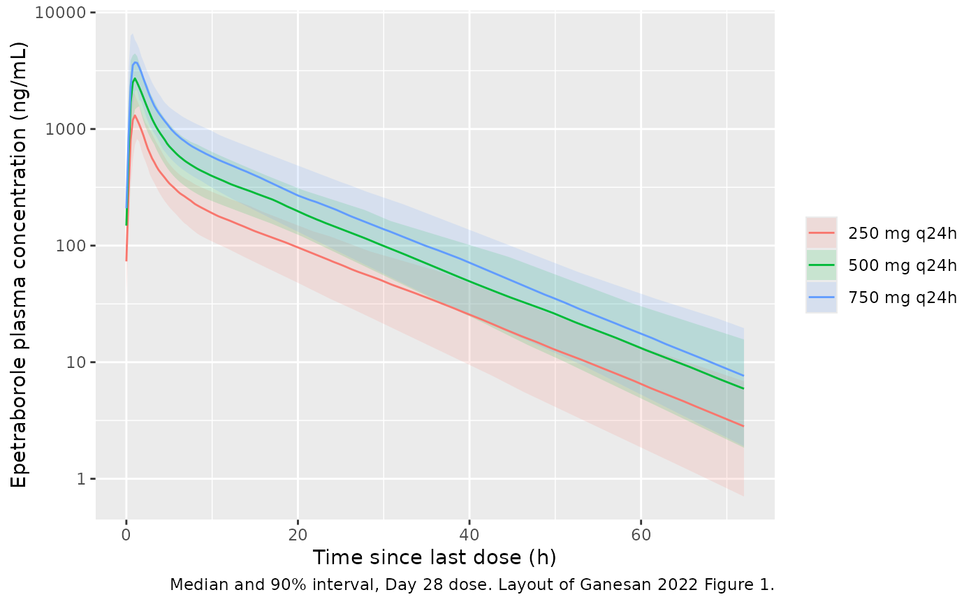

PKNCA validation against the phase 1b study

conc_po <- sim_po |>
  dplyr::filter(!is.na(Cc)) |>
  dplyr::select(id, time, Cc, regimen)
dose_po <- events_po |>
  dplyr::filter(evid == 1) |>
  dplyr::select(id, time, amt, regimen)

nca_day <- function(start, end, regimens, half_life) {
  cc <- conc_po |> dplyr::filter(regimen %in% regimens, time >= start, time <= end)
  dd <- dose_po |> dplyr::filter(regimen %in% regimens, time <= start)
  intervals <- data.frame(start = start, end = start + 24, auclast = TRUE, cmax = TRUE, tmax = TRUE)
  if (half_life) {
    intervals <- dplyr::bind_rows(intervals, data.frame(start = start, end = end, half.life = TRUE))
  }
  # bind_rows leaves NA in the logical columns; PKNCA requires TRUE/FALSE.
  flag_cols <- setdiff(names(intervals), c("start", "end"))
  intervals[flag_cols] <- lapply(intervals[flag_cols], function(x) !is.na(x) & x)
  PKNCA::pk.nca(PKNCA::PKNCAdata(
    PKNCA::PKNCAconc(cc, Cc ~ time | regimen + id),
    PKNCA::PKNCAdose(dd, amt ~ time | regimen + id),
    intervals = intervals
  ))
}
nca_d1 <- nca_day(0, 24, unique(events_po$regimen), half_life = FALSE)
nca_d28 <- nca_day(27 * 24, 27 * 24 + 72, c("250 mg q24h", "500 mg q24h", "750 mg q24h"), half_life = TRUE)

Eckburg 2022 Table 2 reports arithmetic means for AUC0-24, Cmax and half-life and medians for Tmax, in ng/mL; they are converted to mg/L here. The “500 mg q24h” Day 1 row is cohort 3 (n = 6), and “500 mg fed” is the fed arm of cohort 7.

published_d1 <- tibble::tribble(
  ~regimen,      ~auclast, ~cmax, ~tmax,
  "250 mg q24h", 6.95,     1.44,  1.03,
  "500 mg q24h", 12.3,     2.62,  1.0,
  "750 mg q24h", 20.0,     5.60,  1.0,
  "500 mg fed",  11.2,     1.75,  2.0
)
cmp_d1 <- nlmixr2lib::ncaComparisonTable(
  simulated = nca_d1, reference = published_d1, by = "regimen",
  units = c(auclast = "mg*h/L", cmax = "mg/L", tmax = "h"),
  tolerance_pct = 20
)
knitr::kable(cmp_d1, caption = "Day 1, simulated vs. Eckburg 2022 Table 2. * differs by more than 20%.")

Day 1, simulated vs. Eckburg 2022 Table 2. * differs by more than 20%.

NCA parameter	regimen	Reference	Simulated	% diff
Cmax (mg/L)	250 mg q24h	1.44	1.29	-10.6%
Cmax (mg/L)	500 mg q24h	2.62	2.64	+0.7%
Cmax (mg/L)	750 mg q24h	5.6	4	-28.6%*
Cmax (mg/L)	500 mg fed	1.75	1.62	-7.4%
Tmax (h)	250 mg q24h	1.03	1	-2.9%
Tmax (h)	500 mg q24h	1	1	+0.0%
Tmax (h)	750 mg q24h	1	1	+0.0%
Tmax (h)	500 mg fed	2	2.25	+12.5%
AUClast (mg*h/L)	250 mg q24h	6.95	5.53	-20.4%*
AUClast (mg*h/L)	500 mg q24h	12.3	11.4	-7.3%
AUClast (mg*h/L)	750 mg q24h	20	17.1	-14.3%
AUClast (mg*h/L)	500 mg fed	11.2	11.9	+5.8%

published_d28 <- tibble::tribble(
  ~regimen,      ~auclast, ~cmax, ~tmax, ~half.life,
  "250 mg q24h", 7.10,     1.39,  1.5,   10.6,
  "500 mg q24h", 13.7,     2.85,  1.0,   10.2,
  "750 mg q24h", 24.4,     5.28,  1.0,   10.3
)
cmp_d28 <- nlmixr2lib::ncaComparisonTable(
  simulated = nca_d28, reference = published_d28, by = "regimen",
  units = c(auclast = "mg*h/L", cmax = "mg/L", tmax = "h", half.life = "h"),
  tolerance_pct = 20
)
knitr::kable(cmp_d28, caption = "Day 28, simulated vs. Eckburg 2022 Table 2. * differs by more than 20%.")

Day 28, simulated vs. Eckburg 2022 Table 2. * differs by more than 20%.

NCA parameter	regimen	Reference	Simulated	% diff
Cmax (mg/L)	250 mg q24h	1.39	1.37	-1.7%
Cmax (mg/L)	500 mg q24h	2.85	2.8	-1.8%
Cmax (mg/L)	750 mg q24h	5.28	4.08	-22.8%*
Tmax (h)	250 mg q24h	1.5	1	-33.3%*
Tmax (h)	500 mg q24h	1	1	+0.0%
Tmax (h)	750 mg q24h	1	1	+0.0%
AUClast (mg*h/L)	250 mg q24h	7.1	6.47	-8.9%
AUClast (mg*h/L)	500 mg q24h	13.7	13.1	-4.6%
AUClast (mg*h/L)	750 mg q24h	24.4	19.7	-19.4%
t½ (h)	250 mg q24h	10.6	10.3	-3.3%
t½ (h)	500 mg q24h	10.2	10.2	-0.5%
t½ (h)	750 mg q24h	10.3	10.1	-1.7%

# Robust central tendency only: a
# mis-transcribed CL, F, V or dose moves these medians by tens of percent.
res_d1 <- as.data.frame(nca_d1)
med <- function(res, reg, param, start) {
  x <- res$PPORRES[res$regimen == reg & res$PPTESTCD == param & res$start == start]
  stopifnot(length(x) > 0)
  median(x, na.rm = TRUE)
}
res_d28 <- as.data.frame(nca_d28)
stopifnot(
  abs(med(res_d1, "500 mg q24h", "auclast", 0) / 12.3 - 1) < 0.3,
  abs(med(res_d1, "250 mg q24h", "auclast", 0) / 6.95 - 1) < 0.3,
  abs(med(res_d28, "500 mg q24h", "auclast", 648) / 13.7 - 1) < 0.3,
  abs(med(res_d1, "500 mg q24h", "tmax", 0) - 1.0) <= 0.5,
  abs(med(res_d1, "500 mg fed", "tmax", 0) - 2.0) <= 0.75
)

At 250 and 500 mg the simulated Day 1 and Day 28 AUC0-24, Cmax and half-life are within about 20% of the phase 1b means, and Tmax reproduces both the fasted (1.0 h) and fed (2.0 h) medians. The 250 mg Day 28 Tmax median of 1.5 h against 1.0 h simulated is one sampling step on a cohort of five. Two departures follow from the model structure:

• The model is linear in dose, but the observed 750 mg cohort (n = 6) had a Cmax of 5.6 mg/L on Day 1, 1.4 times the dose-proportional value from the 500 mg cohort (2.62 mg/L); the simulated 750 mg Cmax and AUC are therefore 20-29% low. The observed 500 mg Cmax itself ranges from 2.6 to 3.8 mg/L across cohorts 2, 3 and 7.
• Food changes only ka in the model, so the simulated fed AUC equals the fasted AUC. In the phase 1b food-effect cohort the fed AUC0-24 was 26% below the fasted arm (11.2 vs 15.2 mg*h/L); the fed row agrees with the reference only because the comparison fasted value (cohort 3, 12.3) is lower than cohort 7’s.

IV plasma and ELF exposure (Tenero 2013)

n_iv <- 100L
iv_subj <- tibble::tibble(id = seq_len(n_iv), WT = pmin(pmax(rnorm(n_iv, 80, 10), 55), 110))
events_iv <- dplyr::bind_rows(
  iv_subj |> dplyr::mutate(time = 0, amt = 1500, dur = 1, evid = 1L, cmt = "central", dvid = NA_integer_),
  tidyr::crossing(iv_subj, time = c(seq(0, 12, by = 0.25), seq(12.5, 96, by = 0.5))) |>
    dplyr::mutate(amt = NA_real_, dur = NA_real_, evid = 0L, cmt = NA_character_, dvid = 1L)
) |>
  dplyr::mutate(FED = 0L, OCC = 1L, regimen = "1500 mg IV, 1 h") |>
  dplyr::arrange(id, time, dplyr::desc(evid))
sim_iv <- rxode2::rxSolve(mod, events = events_iv, keep = c("regimen", "WT"),
                          returnType = "data.frame")
stopifnot(!anyNA(sim_iv$Cc))

nca_iv <- PKNCA::pk.nca(PKNCA::PKNCAdata(
  PKNCA::PKNCAconc(sim_iv |> dplyr::select(id, time, Cc, regimen), Cc ~ time | regimen + id),
  PKNCA::PKNCAdose(events_iv |> dplyr::filter(evid == 1) |> dplyr::select(id, time, amt, dur, regimen),
                   amt ~ time | regimen + id, duration = "dur", route = "intravascular"),
  intervals = data.frame(start = 0, end = Inf, cmax = TRUE, aucinf.obs = TRUE,
                         cl.obs = TRUE, vss.obs = TRUE, half.life = TRUE)
))
published_iv <- tibble::tribble(
  ~regimen,          ~cmax, ~aucinf.obs, ~cl.obs, ~vss.obs, ~half.life,
  "1500 mg IV, 1 h", 21.6,  65.0,        23.1,    231,      10.7
)
cmp_iv <- nlmixr2lib::ncaComparisonTable(
  simulated = nca_iv, reference = published_iv, by = "regimen",
  units = c(cmax = "mg/L", aucinf.obs = "mg*h/L", cl.obs = "L/h", vss.obs = "L", half.life = "h"),
  tolerance_pct = 20
)
knitr::kable(cmp_iv, caption = "Single 1500 mg IV dose, simulated vs. Tenero 2013 (geometric means; half-life median). * differs by more than 20%.")

Single 1500 mg IV dose, simulated vs. Tenero 2013 (geometric means; half-life median). * differs by more than 20%.

NCA parameter	regimen	Reference	Simulated	% diff
Cmax (mg/L)	1500 mg IV, 1 h	21.6	21.2	-1.8%
AUC0-∞ (obs) (mg*h/L)	1500 mg IV, 1 h	65	71.1	+9.3%
t½ (h)	1500 mg IV, 1 h	10.7	10.5	-1.8%
CL/F (L/h)	1500 mg IV, 1 h	23.1	21.1	-8.6%
Vss/F (L)	1500 mg IV, 1 h	231	227	-1.9%

auc_trap <- function(t, y) sum(diff(t) * (head(y, -1) + tail(y, -1)) / 2)
elf_ratio <- sim_iv |>
  dplyr::group_by(id) |>
  dplyr::summarise(ratio = auc_trap(time, Celf) / auc_trap(time, Cc), .groups = "drop")
# Penetration ratio of the mean profiles, the way Tenero computed it from one
# bronchoscopy per subject at 2, 6 or 12 h.
mean_prof <- sim_iv |>
  dplyr::group_by(time) |>
  dplyr::summarise(Cc = mean(Cc), Celf = mean(Celf), .groups = "drop")
elf_summary <- data.frame(
  quantity = c("Median individual ELF:plasma AUC ratio", "Ratio of mean-profile AUCs", "Tenero 2013 (AUC-based)"),
  value = c(median(elf_ratio$ratio), auc_trap(mean_prof$time, mean_prof$Celf) / auc_trap(mean_prof$time, mean_prof$Cc), 0.538)
)
elf_summary |>
  dplyr::rename("Quantity" = quantity, "ELF:plasma ratio" = value) |>
  knitr::kable(digits = 2)

Quantity	ELF:plasma ratio
Median individual ELF:plasma AUC ratio	0.38
Ratio of mean-profile AUCs	0.41
Tenero 2013 (AUC-based)	0.54

iv_res <- as.data.frame(nca_iv)
stopifnot(
  abs(median(iv_res$PPORRES[iv_res$PPTESTCD == "cl.obs"]) / 21.9 - 1) < 0.25,
  abs(median(elf_ratio$ratio) - 0.40) < 0.1
)

The simulated IV Cmax, AUC, clearance, Vss and half-life are all within 10% of Tenero 2013 (the comparison table labels clearance and Vss “/F”, its generic header; for an IV dose F = 1). The simulated ELF:plasma AUC ratio (about 0.4, individual or mean-profile) is a quarter below Tenero’s 0.54, which was computed from one bronchoscopy per subject at 2, 6 or 12 h.

Assumptions and deviations

• Transit compartments. Not printed; two compartments, each at the fed or fasted ka, chosen because they alone reproduce both phase 1b Tmax medians (section above).
• ELF compartment depletes plasma. Not stated; chosen from the NONMEM general-linear meaning of K14 / K40 and because only this reading reproduces Tenero 2013’s IV clearance (section above). With the non-depleting link reading the model would under-predict IV clearance by about 25%.
• ELF concentration = ELF amount / Vc. No ELF volume is printed; Vc is the only scaling that needs no extra parameter.
• Logit-normal IIV on F. The scale is not stated; logit is chosen because it reproduces the observed phase 1b AUC variability and keeps F below 1 (section above).
• Allometric exponents. Not printed. The parameter units (per 70 kg) and the “allometric scaling approach” in the Results point to the standard fixed exponents, 0.75 for CL, CLd and CLd2 and 1 for Vc, Vp and Vp2. K14, K40 and ka are reported in 1/h without a weight normalisation and are not scaled.
• IIV on ka. Table 2 prints the 29.5% IIV on the Ka, fast row only; one eta is shared by the fed and fasted ka, the usual NONMEM coding for a covariate-switched parameter.
• Occasions. The source does not define the two occasions of the IOV on ka. The simulations use occasion 1 for the first dosing day and 2 for all later days.
• Food. Food changes only the absorption rate in the model, so the phase 1b fed arm’s lower AUC (26% below fasted) is not reproduced.
• Virtual cohorts. No demographics are reported. Phase 1b subjects are drawn with weight N(75, 12) kg truncated to 45-100 kg (the study admitted 40-100 kg); Tenero 2013 subjects with N(80, 10) kg truncated to 55-110 kg (BMI 24-27 kg/m^2, 93% male).
• No erratum was found for the abstract or poster as of 2026-10-10.