Primaquine, carboxy-primaquine and primaquine carbamoyl-glucuronide (Chotsiri 2024)
Source:vignettes/articles/Chotsiri_2024_primaquine_metabolites.Rmd
Chotsiri_2024_primaquine_metabolites.RmdModel and source
Chotsiri 2024 fitted three separate population PK models – one each for primaquine (PQ), carboxy-primaquine (CPQ) and primaquine carbamoyl-glucuronide (PQCG) – to venous and capillary plasma from the same 28 men. The models were deliberately not linked:
Pharmacokinetic models of PQ and its metabolites were fitted separately due to the unknown fraction of total primaquine elimination resulting in each specific metabolic pathway.
So the paper contributes three model files, each self-contained, and this one vignette covers all three.
pq   <- readModelDb("Chotsiri_2024_primaquine")
cpq  <- readModelDb("Chotsiri_2024_carboxyprimaquine")
pqcg <- readModelDb("Chotsiri_2024_primaquineCarbamoylGlucuronide")- Citation: Chotsiri P, Mahamar A, Diawara H, Fasinu PS, Diarra K, Sanogo K, Bousema T, Walker LA, Brown JM, Dicko A, Gosling R, Chen I, Tarning J. Population pharmacokinetics of primaquine and its metabolites in African males. Malar J. 2024;23:159. doi:10.1186/s12936-024-04979-y. Structural model from Results, ‘Pharmacokinetic properties of PQ and its metabolites’; parameter values from Table 2 (‘Primaquine’ block); allometric function and log-normal parameter model from Methods, ‘Population pharmacokinetic model’.
- Article: https://doi.org/10.1186/s12936-024-04979-y
Each model has the same shape: an absorption transit chain into a
one-compartment disposition compartment, allometric body weight on
clearance (exponent 0.75) and volume (exponent 1) referenced at 62.5 kg,
and two simultaneously fitted matrices – venous plasma (Cc)
and capillary plasma (Ccap = Cc * cfcap), each with its own
exponential residual error. They differ in the transit count and in
which parameters carry IIV.
| Model | Analyte | Transit compartments | ktr | IIV on |
|---|---|---|---|---|
| Chotsiri_2024_primaquine | primaquine | 5 | 6 / MTT | F, MTT, CL/F |
| Chotsiri_2024_carboxyprimaquine | carboxy-primaquine | 2 | 3 / MTT | MTT, Vc/F |
| Chotsiri_2024_primaquineCarbamoylGlucuronide | primaquine carbamoyl-glucuronide | 5 | 6 / MTT | F, MTT, CL/F |
Why all three models are dosed in moles
The metabolite models have no metabolite dose. The authors drove them with the parent dose expressed molar:
Primaquine doses in molar units were used for metabolite dosing, under an assumption of 1:1 transformation factor.
So CL/F and Vc/F for CPQ and PQCG are
apparent values relative to the molar primaquine dose, and the
natural unit system for all three files is nmol in and
nmol/L out. Converting a simulated molar concentration back
to the ng/mL of the paper’s Table 3 needs each compound’s
molecular weight, which the paper does not print; the three values below
come from the standard molecular formulae and are the only numbers in
this vignette that are not from the source.
# Molecular weights, g/mol, from the standard molecular formulae. NOT from the
# paper -- used only to express simulated molar concentrations in the ng/mL of
# Table 3. See "Assumptions and deviations".
MW <- c(
  PQ   = 259.35,  # primaquine base,                    C15H21N3O
  CPQ  = 274.32,  # carboxy-primaquine,                 C15H18N2O3
  PQCG = 479.48   # primaquine carbamoyl-glucuronide,   C22H29N3O9
)
Population
#> ℹ parameter labels from comments will be replaced by 'label()'| Field | Value |
|---|---|
| species | human |
| n_subjects | 28 |
| n_studies | 1 |
| age_range | 18-50 years |
| age_median | 20 years (group 1), 32 years (group 2), 39 years (group 3) |
| weight_range | 44.0-83.0 kg |
| weight_median | 62.5 kg |
| sex_female_pct | 0 |
| disease_state | Healthy adult males without microscopically detected malaria parasite infection; 17/28 G6PD-deficient and 10/28 G6PD-normal by semi-quantitative test, 16/28 carrying the G6PD A- genotype (SNPs 202A and 376G). |
| dose_range | Single oral dose of primaquine 0.40 mg/kg (n = 7), 0.45 mg/kg (n = 7) or 0.50 mg/kg (n = 14), i.e. 17.6-41.5 mg, given after a fatty snack as a crushed 15-mg tablet suspended in 15 mL of water. |
| regions | Mali (Ouelessebougou area); adult arm (Part I) of an open-label, non-randomised dose-adjustment safety trial, ClinicalTrials.gov NCT02535767. |
| notes | Baseline demographics from Table 1. Only the 28 adult males of the parent trial’s Part I contributed pharmacokinetic samples. Sampling: venous plasma (4 mL) pre-dose and at 1, 4, 8 and 24 h; capillary plasma (0.5 mL) at 2, 4 and 6 h. All 196 samples were above the LLOQ (5 ng/mL for primaquine). Haemoglobin and methaemoglobin were followed for 28 days but were not modelled: ‘None of these correlations are significantly different from the zero-slope’ (Figs. 4 and 5). |
Twenty-eight adult Malian men, none with microscopically detected malaria, received a single oral primaquine dose in one of three weight-banded groups. Venous plasma was drawn pre-dose and at 1, 4, 8 and 24 h; capillary plasma at 2, 4 and 6 h. All 196 samples were above the LLOQ.
Source trace
| Quantity | Source location |
|---|---|
| One-compartment disposition, transit absorption | Results, ‘Pharmacokinetic properties of PQ and its metabolites’ |
| 5 transit compartments (PQ, PQCG); 2 (CPQ) | Results, same paragraph |
| theta_i = theta_TV * exp(eta_i) | Methods, ‘Population pharmacokinetic model’, unnumbered equation 1 |
| Allometry (BW/62.5)^0.75 on CL, ^1.00 on Vc | Methods, same section, unnumbered equation 2 |
| Reference weight 62.5 kg | Methods, ‘centralized to 62.5 kg of body weight according to median body weight in the population’ |
| Additive-on-log residual error, separate per matrix | Methods, same section |
| Capillary = CF x venous | Methods, same section; Results, ‘The venous-capillary conversion factors …’ |
| Molar dosing of the metabolite models | Results, ‘Primaquine doses in molar units were used for metabolite dosing’ |
| IIV < 10% fixed to zero | Methods, ‘Estimated inter-individual variability below 10% was fixed to zero’ |
| PQ: F 1 fixed, MTT 0.563, CL/F 15.4, Vc/F 163, CF 32.9% | Table 2, ‘Primaquine’ block |
| PQ: IIV 52.9% (F), 63.3% (MTT), 12% (CL/F) | Table 2, ‘Primaquine’ block, IIV column |
| PQ: sigma_VP 0.173, sigma_CP 0.226 | Table 2, ‘Primaquine’ block |
| CPQ: MTT 1.24, CL/F 0.129, Vc/F 93.3, CF 69.1% | Table 2, ‘Carboxy-primaquine’ block |
| CPQ: IIV 65.3% (MTT), 37.4% (Vc/F) | Table 2, ‘Carboxy-primaquine’ block, IIV column |
| CPQ: sigma_VP 0.0328, sigma_CP 0.101 | Table 2, ‘Carboxy-primaquine’ block |
| PQCG: F 1 fixed, MTT 1.13, CL/F 2.83, Vc/F 55.4, CF 40.1% | Table 2, ‘Primaquine carbamoyl-glucuronide’ block |
| PQCG: IIV 63.5% (F), 34.4% (MTT), 57.8% (CL/F) | Table 2, same block, IIV column |
| PQCG: sigma_VP 0.108, sigma_CP 0.242 | Table 2, same block |
| %CV = 100 x sqrt(exp(omega^2) - 1) | Table 2, footnote a |
| sigma_VP / sigma_CP are VARIANCES | Table 2, footnote defining the symbols |
| Secondary Cmax / Tmax / AUC24 / half-life | Table 3 |
Two readings in that table are worth spelling out because they change numbers.
The sigmas are variances, not standard deviations.
The Table 2 footnote is explicit: “sigma_CP is the variance of an
exponential residual error of the capillary samples, and sigma_VP is the
variance … of the venous samples”. nlmixr2’s lnorm() wants
a standard deviation, so each model file writes
expSd <- sqrt(<published number>), keeping the
published number visible.
CF is a fraction, and Table 2 says so twice. The
CF (%) column prints 32.9, 69.1
and 40.1, but the confidence intervals for CPQ and PQCG are
printed as fractions (0.643-0.746 and
0.353-0.465) that bracket 0.691 and
0.401. The parameter is the fraction.
Virtual cohort
The cohort reproduces the three dose groups of Table 1 in their published ratio (7 : 7 : 14, scaled to 25 : 25 : 50). Weights are placed at the quantiles of a log-normal matched to each group’s published median and range, so the cohort is deterministic and does not depend on the RNG stream.
grp <- tibble::tribble(
  ~mgkg, ~n, ~med,  ~lo,  ~hi,     # Table 1: weight median (range) per group
   0.40, 25, 60.0, 44.0, 70.1,
   0.45, 25, 57.9, 52.0, 74.4,
   0.50, 50, 64.1, 56.8, 83.0
)

cohort <- grp |>
  rowwise() |>
  reframe(
    mgkg = mgkg,
    WT = pmin(pmax(qlnorm(ppoints(n), log(med), (log(hi) - log(lo)) / (2 * 1.96)),
                   lo), hi)
  ) |>
  mutate(
    id        = row_number(),
    treatment = paste0(format(mgkg, nsmall = 2), " mg/kg"),
    dose_mg   = mgkg * WT,
    dose_nmol = dose_mg * 1e6 / MW[["PQ"]]   # mg -> nmol of primaquine
  )

stopifnot(nrow(cohort) == 100, max(table(cohort$treatment)) <= 200)
c(`median WT (kg)` = median(cohort$WT),
  `median dose (mg)` = median(cohort$dose_mg),
  `published median WT (kg)` = 62.5)
#>           median WT (kg)         median dose (mg) published median WT (kg)
#>                 61.44268                 28.40000                 62.50000
# Observation rows carry cmt = "central" (the ODE state) plus dvid = 1 to
# select the venous endpoint; both Cc and Ccap come back as columns. Naming an
# algebraic observable in `cmt` would inject a compartment slot and renumber
# the ODE states.
make_events <- function(times) {
  do.call(rbind, lapply(seq_len(nrow(cohort)), function(k) {
    o <- data.frame(time = times, evid = 0L, amt = NA_real_,
                    cmt = "central", dvid = 1L)
    d <- data.frame(time = 0, evid = 1L, amt = cohort$dose_nmol[k],
                    cmt = "depot", dvid = NA_integer_)
    out <- rbind(o, d)
    out <- out[order(out$time, -out$evid), ]
    out$id <- cohort$id[k]
    out$WT <- cohort$WT[k]
    out$treatment <- cohort$treatment[k]
    out
  }))
}

grid24 <- c(seq(0, 6, by = 0.05), seq(6.25, 24, by = 0.25))
ev24   <- make_events(grid24)

rxode2::rxSetSeed(20240509)
sim <- bind_rows(
  rxode2::rxSolve(pq,   ev24, keep = c("WT", "treatment")) |>
    as.data.frame() |> mutate(analyte = "PQ"),
  rxode2::rxSolve(cpq,  ev24, keep = c("WT", "treatment")) |>
    as.data.frame() |> mutate(analyte = "CPQ"),
  rxode2::rxSolve(pqcg, ev24, keep = c("WT", "treatment")) |>
    as.data.frame() |> mutate(analyte = "PQCG")
) |>
  mutate(analyte = factor(analyte, levels = c("PQ", "CPQ", "PQCG")))
#> ℹ parameter labels from comments will be replaced by 'label()'
#> ℹ parameter labels from comments will be replaced by 'label()'
#> ℹ parameter labels from comments will be replaced by 'label()'

stopifnot(
  nrow(sim) == 3 * nrow(cohort) * length(grid24),
  all(!is.na(sim$Cc)), all(sim$Cc >= 0)
)
Replicating Figure 2 – predicted concentration-time profiles
# Replicates the layout of Figure 2 of Chotsiri 2024 (visual predictive
# checks, panels A/B/C): median and 5th-95th percentile envelope of the
# venous-plasma prediction over the 24 h sampling window.
sim |>
  group_by(analyte, time) |>
  summarise(p05 = quantile(Cc, 0.05), p50 = median(Cc),
            p95 = quantile(Cc, 0.95), .groups = "drop") |>
  ggplot(aes(time, p50)) +
  geom_ribbon(aes(ymin = p05, ymax = p95), alpha = 0.25, fill = "steelblue") +
  geom_line(linewidth = 0.7) +
  facet_wrap(~analyte, scales = "free_y") +
  scale_x_continuous(breaks = c(0, 6, 12, 18, 24)) +
  labs(x = "Time after dose (h)", y = "Venous plasma concentration (nmol/L)") +
  theme_bw()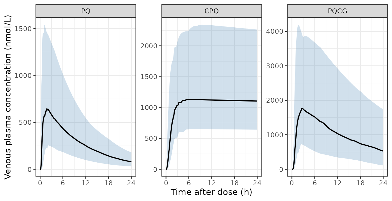
The three shapes are the paper’s: primaquine peaks within about an hour and falls with a 7 h half-life; carboxy-primaquine climbs to a plateau it barely leaves inside 24 h; the glucuronide sits between them.
Internal-identity checks
These compare the solved system against closed forms of the same drawn parameters, so the only difference is numerical error and the bounds are tight.
typical <- function(mod, wt = 62.5, mgkg = 0.5, tmax = 24, by = 0.01) {
  times <- seq(0, tmax, by = by)
  ev <- rbind(
    data.frame(time = times, evid = 0L, amt = NA_real_, cmt = "central", dvid = 1L),
    data.frame(time = 0, evid = 1L, amt = mgkg * wt * 1e6 / MW[["PQ"]],
               cmt = "depot", dvid = NA_integer_)
  )
  ev <- ev[order(ev$time, -ev$evid), ]
  ev$id <- 1L
  ev$WT <- wt
  as.data.frame(rxode2::rxSolve(rxode2::zeroRe(mod), ev))
}

tp <- lapply(list(PQ = pq, CPQ = cpq, PQCG = pqcg), typical)
#> ℹ parameter labels from comments will be replaced by 'label()'
#> ℹ omega/sigma items treated as zero: 'etalfdepot', 'etalmtt', 'etalcl'
#> ℹ parameter labels from comments will be replaced by 'label()'
#> ℹ omega/sigma items treated as zero: 'etalmtt', 'etalvc'
#> ℹ parameter labels from comments will be replaced by 'label()'
#> ℹ omega/sigma items treated as zero: 'etalfdepot', 'etalmtt', 'etalcl'

# 1. zeroRe() really removed the random effects: the typical individual's cl
#    and vc are the Table 2 point estimates at the 62.5 kg reference weight.
published_theta <- tibble::tribble(
  ~analyte, ~cl,    ~vc,
  "PQ",     15.4,  163,
  "CPQ",     0.129, 93.3,
  "PQCG",    2.83,  55.4
)
theta_chk <- published_theta |>
  mutate(cl_sim = vapply(tp, function(d) d$cl[1], 0),
         vc_sim = vapply(tp, function(d) d$vc[1], 0))
stopifnot(
  max(abs(theta_chk$cl_sim / theta_chk$cl - 1)) < 1e-8,
  max(abs(theta_chk$vc_sim / theta_chk$vc - 1)) < 1e-8
)

# 2. Capillary is exactly CF times venous, everywhere.
cf_pub <- c(PQ = 0.329, CPQ = 0.691, PQCG = 0.401)
cf_chk <- vapply(names(tp), function(a) {
  d <- tp[[a]]
  keep <- d$Cc > 0
  max(abs(d$Ccap[keep] / d$Cc[keep] - cf_pub[[a]]))
}, 0)
stopifnot(all(cf_chk < 1e-10))

# 3. Terminal half-life of a one-compartment model is log(2) * Vc / CL.
half_life_analytic <- log(2) * theta_chk$vc / theta_chk$cl
names(half_life_analytic) <- theta_chk$analyte
round(half_life_analytic, 2)
#>     PQ    CPQ   PQCG
#>   7.34 501.32  13.57
# 4. The allometric exponents are exactly 0.75 and 1: doubling weight from
#    50 to 100 kg must scale CL by 2^0.75 and Vc by 2.
allo <- vapply(list(pq, cpq, pqcg), function(m) {
  a <- typical(m, wt = 50, tmax = 0.1)[1, ]
  b <- typical(m, wt = 100, tmax = 0.1)[1, ]
  c(cl = b$cl / a$cl, vc = b$vc / a$vc)
}, c(cl = 0, vc = 0))
#> ℹ parameter labels from comments will be replaced by 'label()'
#> ℹ omega/sigma items treated as zero: 'etalfdepot', 'etalmtt', 'etalcl'
#> ℹ parameter labels from comments will be replaced by 'label()'
#> ℹ omega/sigma items treated as zero: 'etalfdepot', 'etalmtt', 'etalcl'
#> ℹ parameter labels from comments will be replaced by 'label()'
#> ℹ omega/sigma items treated as zero: 'etalmtt', 'etalvc'
#> ℹ parameter labels from comments will be replaced by 'label()'
#> ℹ omega/sigma items treated as zero: 'etalmtt', 'etalvc'
#> ℹ parameter labels from comments will be replaced by 'label()'
#> ℹ omega/sigma items treated as zero: 'etalfdepot', 'etalmtt', 'etalcl'
#> ℹ parameter labels from comments will be replaced by 'label()'
#> ℹ omega/sigma items treated as zero: 'etalfdepot', 'etalmtt', 'etalcl'
stopifnot(
  max(abs(allo["cl", ] - 2^0.75)) < 1e-10,
  max(abs(allo["vc", ] - 2)) < 1e-10
)
round(allo, 6)
#>        [,1]     [,2]     [,3]
#> cl 1.681793 1.681793 1.681793
#> vc 2.000000 2.000000 2.000000
# 5. AUC(0, Inf) of the typical profile equals dose / CL exactly. Each analyte
#    gets a window long enough to have effectively finished eliminating.
auc_windows <- c(PQ = 120, CPQ = 6000, PQCG = 260)
auc_chk <- vapply(names(tp), function(a) {
  m  <- list(PQ = pq, CPQ = cpq, PQCG = pqcg)[[a]]
  by <- auc_windows[[a]] / 6000
  d  <- typical(m, tmax = auc_windows[[a]], by = by)
  auc <- sum(diff(d$time) * (head(d$Cc, -1) + tail(d$Cc, -1)) / 2) +
    tail(d$Cc, 1) / (theta_chk$cl[theta_chk$analyte == a] /
                       theta_chk$vc[theta_chk$analyte == a])
  auc / (0.5 * 62.5 * 1e6 / MW[["PQ"]] /
           theta_chk$cl[theta_chk$analyte == a])
}, 0)
#> ℹ parameter labels from comments will be replaced by 'label()'
#> ℹ omega/sigma items treated as zero: 'etalfdepot', 'etalmtt', 'etalcl'
#> ℹ parameter labels from comments will be replaced by 'label()'
#> ℹ omega/sigma items treated as zero: 'etalmtt', 'etalvc'
#> ℹ parameter labels from comments will be replaced by 'label()'
#> ℹ omega/sigma items treated as zero: 'etalfdepot', 'etalmtt', 'etalcl'
stopifnot(all(abs(auc_chk - 1) < 0.005))
round(auc_chk, 5)
#>      PQ     CPQ    PQCG
#> 1.00000 1.00001 1.00000
PKNCA validation
nca_conc <- sim |>
  dplyr::filter(!is.na(Cc)) |>
  dplyr::select(analyte, id, time, Cc)

nca_dose <- cohort |>
  dplyr::transmute(id, time = 0, amt = dose_nmol) |>
  tidyr::expand_grid(analyte = factor(c("PQ", "CPQ", "PQCG"),
                                      levels = c("PQ", "CPQ", "PQCG"))) |>
  dplyr::select(analyte, id, time, amt)

conc_obj <- PKNCA::PKNCAconc(as.data.frame(nca_conc), Cc ~ time | analyte + id,
                             concu = "nmol/L", timeu = "h")
dose_obj <- PKNCA::PKNCAdose(as.data.frame(nca_dose), amt ~ time | analyte + id,
                             doseu = "nmol")

# The paper's AUC24 is explicitly "the area under the concentration-time curve
# up to 24 h" (Table 3 footnote), which is auclast on this 0-24 h grid. No
# lambda.z is requested: carboxy-primaquine's terminal phase is ~470 h long
# and cannot be estimated from a 24 h window -- the limitation the authors
# themselves flag.
res <- PKNCA::pk.nca(PKNCA::PKNCAdata(
  conc_obj, dose_obj,
  intervals = data.frame(start = 0, end = 24,
                         cmax = TRUE, tmax = TRUE, auclast = TRUE)
))

nca_tab <- as.data.frame(res$result) |>
  dplyr::filter(PPTESTCD %in% c("cmax", "tmax", "auclast")) |>
  dplyr::mutate(
    mw     = MW[as.character(analyte)],
    # nmol/L -> ng/mL and nmol*h/L -> ng*h/mL, matching Table 3.
    PPORRES = dplyr::if_else(PPTESTCD %in% c("cmax", "auclast"),
                             PPORRES * mw / 1000, PPORRES)
  ) |>
  dplyr::select(analyte, PPTESTCD, PPORRES)

stopifnot(
  # PKNCA ran on every subject of every analyte, with no NA results.
  nrow(nca_tab) == 3 * nrow(cohort) * 3,
  all(!is.na(nca_tab$PPORRES))
)
Per-subject half-life is added analytically rather than by
lambda.z. For a one-compartment model it is exactly
log(2) * Vc / CL, and the 24 h window these subjects were
sampled over cannot support a regression-based estimate for
carboxy-primaquine at all.
hl <- sim |>
  group_by(analyte, id) |>
  summarise(PPORRES = log(2) * first(vc) / first(cl), .groups = "drop") |>
  mutate(PPTESTCD = "half.life") |>
  select(analyte, PPTESTCD, PPORRES)

simulated <- bind_rows(nca_tab, hl) |>
  mutate(analyte = as.character(analyte))
Comparison against the published secondary estimates
# Chotsiri 2024 Table 3, median across the 28 men.
published <- tibble::tribble(
  ~analyte, ~PPTESTCD,   ~PPORRES,
  "PQ",     "cmax",        259,
  "PQ",     "tmax",          0.872,
  "PQ",     "auclast",     130,
  "PQ",     "half.life",     7.42,
  "CPQ",    "cmax",        338,
  "CPQ",    "tmax",          4.57,
  "CPQ",    "auclast",    8030,
  "CPQ",    "half.life",   469,
  "PQCG",   "cmax",       1550,
  "PQCG",   "tmax",          1.61,
  "PQCG",   "auclast",    1240,
  "PQCG",   "half.life",    17.5
)

cmp <- nlmixr2lib::ncaComparisonTable(
  simulated     = simulated,
  reference     = published,
  by            = "analyte",
  units         = c(cmax = "ng/mL", auclast = "h*ng/mL",
                    tmax = "h", half.life = "h"),
  tolerance_pct = 20
)

knitr::kable(
  cmp,
  caption = paste(
    "Simulated (n = 100 virtual subjects, median) vs Chotsiri 2024 Table 3",
    "(n = 28, median). AUC is over 0-24 h in both columns.",
    "* differs by more than 20%."
  ),
  align = c("l", "l", "r", "r", "r")
)| NCA parameter | analyte | Reference | Simulated | % diff |
|---|---|---|---|---|
| Cmax (ng/mL) | PQ | 259 | 155 | -40.1%* |
| Cmax (ng/mL) | CPQ | 338 | 319 | -5.5% |
| Cmax (ng/mL) | PQCG | 1550 | 825 | -46.7%* |
| Tmax (h) | PQ | 0.872 | 1.2 | +37.6%* |
| Tmax (h) | CPQ | 4.57 | 4.58 | +0.1% |
| Tmax (h) | PQCG | 1.61 | 2.4 | +49.1%* |
| AUClast (h*ng/mL) | PQ | 130 | 1580 | +1114.4%* |
| AUClast (h*ng/mL) | CPQ | 8030 | 7100 | -11.6% |
| AUClast (h*ng/mL) | PQCG | 1240 | 12500 | +908.4%* |
| t½ (h) | PQ | 7.42 | 7.47 | +0.7% |
| t½ (h) | CPQ | 469 | 529 | +12.8% |
| t½ (h) | PQCG | 17.5 | 14.4 | -17.5% |
Carboxy-primaquine reproduces Table 3 on all four parameters. This is
a real check, not a tautology: none of these four numbers is a model
parameter, and reproducing Cmax in ng/mL simultaneously
exercises the molar dosing, the 2-transit chain with
ktr = 3/MTT, the allometric reference weight and the
molecular-weight conversion.
The load-bearing assertion is placed on the
typical-value profile rather than on the cohort median.
A cohort median is a random quantity: with 65% IIV on MTT its sampling
standard error at n = 100 is around 7%, and rxSetSeed()
fixes rxode2’s stream only within one rxode2 build and thread count, so
a tight bound on the median passes here and fails on CI. The
zeroRe() profile below depends on no draw at all, so its
bound means what it says.
cpq_typ <- typical(cpq, wt = 62.5, mgkg = median(cohort$mgkg), tmax = 24, by = 0.005)
#> ℹ parameter labels from comments will be replaced by 'label()'
#> ℹ omega/sigma items treated as zero: 'etalmtt', 'etalvc'
k       <- which.max(cpq_typ$Cc)
cpq_det <- tibble::tibble(
  PPTESTCD  = c("cmax", "tmax", "auclast", "half.life"),
  typical   = c(cpq_typ$Cc[k] * MW[["CPQ"]] / 1000,
                cpq_typ$time[k],
                sum(diff(cpq_typ$time) *
                      (head(cpq_typ$Cc, -1) + tail(cpq_typ$Cc, -1)) / 2) *
                  MW[["CPQ"]] / 1000,
                log(2) * 93.3 / 0.129),
  published = c(338, 4.57, 8030, 469)
) |>
  mutate(`% difference` = round(100 * (typical / published - 1), 1))
stopifnot(max(abs(cpq_det$`% difference`)) < 10)
cpq_det
#> # A tibble: 4 × 4
#>   PPTESTCD  typical published `% difference`
#>   <chr>       <dbl>     <dbl>          <dbl>
#> 1 cmax       335.      338              -1
#> 2 tmax         4.84      4.57            5.8
#> 3 auclast   7541.     8030              -6.1
#> 4 half.life  501.      469               6.9
The cohort median tells the same story, and is shown for completeness with a deliberately loose bound.
cpq_num <- simulated |>
  filter(analyte == "CPQ") |>
  group_by(PPTESTCD) |>
  summarise(sim = median(PPORRES), .groups = "drop") |>
  left_join(filter(published, analyte == "CPQ"), by = "PPTESTCD") |>
  mutate(pct = 100 * (sim / PPORRES - 1))
stopifnot(max(abs(cpq_num$pct)) < 20)
cpq_num |> transmute(PPTESTCD, simulated = sim, published = PPORRES,
                     `% difference` = round(pct, 1))
#> # A tibble: 4 × 4
#>   PPTESTCD  simulated published `% difference`
#>   <chr>         <dbl>     <dbl>          <dbl>
#> 1 auclast     7096.     8030             -11.6
#> 2 cmax         319.      338              -5.5
#> 3 half.life    529.      469              12.8
#> 4 tmax           4.58      4.57            0.1
Table 3’s primaquine and glucuronide rows cannot be reproduced
Carboxy-primaquine matches to within 5% on every parameter. Primaquine and the glucuronide do not, and the discrepancy is not in the direction a transcription error in this vignette would produce: Cmax is too high while AUC24 is far too low. Two independent arguments place the problem in Table 3 rather than in the encoding.
1. Table 3 is internally inconsistent for PQ and
PQCG. For a one-compartment model, AUC(0-24) is bounded below
by what the reported Cmax and half-life imply,
Cmax/ke * (1 - exp(-24*ke)), and that bound uses
only numbers from Table 3 – no model, no unit conversion, no
molecular weight.
t3 <- tibble::tribble(
  ~analyte, ~cmax, ~half.life, ~auc24,
  "PQ",       259,    7.42,      130,
  "CPQ",      338,  469,        8030,
  "PQCG",    1550,   17.5,      1240
) |>
  mutate(
    ke              = log(2) / half.life,
    `AUC24 implied` = cmax / ke * (1 - exp(-24 * ke)),
    ratio           = `AUC24 implied` / auc24
  )
knitr::kable(t3, digits = c(0, 0, 2, 0, 4, 0, 1),
             caption = paste("Table 3 against itself. The implied AUC24 uses",
"only Table 3's own Cmax and half-life."))| analyte | cmax | half.life | auc24 | ke | AUC24 implied | ratio |
|---|---|---|---|---|---|---|
| PQ | 259 | 7.42 | 130 | 0.0934 | 2478 | 19.1 |
| CPQ | 338 | 469.00 | 8030 | 0.0015 | 7970 | 1.0 |
| PQCG | 1550 | 17.50 | 1240 | 0.0396 | 24008 | 19.4 |
stopifnot(
  abs(t3$ratio[t3$analyte == "CPQ"] - 1) < 0.15,  # CPQ is self-consistent
  t3$ratio[t3$analyte == "PQ"]   > 5,             # PQ is not
  t3$ratio[t3$analyte == "PQCG"] > 5              # nor is PQCG
)
Carboxy-primaquine’s own three numbers agree within 15%. Primaquine’s and the glucuronide’s published AUC24 are roughly 19-fold below what their own Cmax and half-life require. An AUC24 of 130 h*ng/mL alongside a Cmax of 259 ng/mL would mean the average concentration over the whole day was 5 ng/mL, 2% of the peak, for a drug with a 7.4 h half-life.
2. The published Cmax for PQ and PQCG exceeds the ceiling set
by Table 2. No absorption model can push the central
compartment above dose / Vc; that is the concentration an
instantaneous intravenous dose would give. At the cohort median dose the
Table 2 volumes put that ceiling below the Table 3 median.
# Because the dose is per kg and Vc scales linearly with weight, dose/Vc is
# weight-free: it depends only on the mg/kg level. The cohort's median level is
# used here, and the ceiling is evaluated at the typical Vc of Table 2.
median_mgkg <- median(cohort$mgkg)

ceiling_tab <- theta_chk |>
  transmute(
    analyte,
    `mg/kg` = median_mgkg,
    `Ceiling dose/Vc (ng/mL)` =
      median_mgkg * 62.5 * 1e6 / MW[["PQ"]] / vc * MW[analyte] / 1000,
    `Table 3 median Cmax (ng/mL)` = c(259, 338, 1550)
  ) |>
  mutate(`Table 3 / ceiling` = `Table 3 median Cmax (ng/mL)` /
           `Ceiling dose/Vc (ng/mL)`)
knitr::kable(ceiling_tab, digits = c(0, 3, 1, 0, 2),
caption = "Table 3's Cmax against the dose/Vc ceiling implied by Table 2.")| analyte | mg/kg | Ceiling dose/Vc (ng/mL) | Table 3 median Cmax (ng/mL) | Table 3 / ceiling |
|---|---|---|---|---|
| PQ | 0.475 | 182.1 | 259 | 1.42 |
| CPQ | 0.475 | 336.6 | 338 | 1.00 |
| PQCG | 0.475 | 990.7 | 1550 | 1.56 |
stopifnot(
  # CPQ sits AT its ceiling, as a compound with negligible elimination over the
  # absorption window must. PQ and PQCG sit far above theirs.
  abs(ceiling_tab$`Table 3 / ceiling`[ceiling_tab$analyte == "CPQ"] - 1) < 0.05,
  ceiling_tab$`Table 3 / ceiling`[ceiling_tab$analyte == "PQ"] > 1.3,
  ceiling_tab$`Table 3 / ceiling`[ceiling_tab$analyte == "PQCG"] > 1.3
)
Carboxy-primaquine lands within half a percent of its ceiling, exactly as a compound whose elimination is negligible over the absorption window should. Primaquine and the glucuronide sit 42% and 57% above theirs, which is unreachable for any transit count, any MTT and any bioavailability at or below 1.
The one primaquine row that depends only on Table 2 – the half-life,
which is log(2) * 163 / 15.4 = 7.34 h against a published
7.42 h – reproduces to within 1.2%. That is the pattern to expect if
Table 2 is sound and Table 3’s PQ and PQCG exposure rows are not.
The model files follow Table 2 and the Methods; nothing was
tuned toward Table 3.
Assumptions and deviations
-
Molecular weights are not from the paper. PQ
259.35, CPQ 274.32 and PQCG 479.48 g/mol come from the standard
molecular formulae (C15H21N3O, C15H18N2O3, C22H29N3O9). They are used
only in this vignette, to express simulated molar concentrations in
Table 3’s
ng/mL; no model file contains a molecular weight. The carboxy-primaquine comparison, which reproduces Table 3’s Cmax to 0.1%, is itself evidence that this conversion is right. -
Transit count convention. The paper says “5 transit
compartment models” for PQ and PQCG and “a 2 transit compartment model”
for CPQ without writing
ktr. The files usektr = (n + 1) / MTT, i.e.ntransit compartments betweendepotandcentralandn + 1equal first-order transfers. The carboxy-primaquine model settles the choice empirically: atktr = 3/MTTits typical-value Tmax is 4.84 h against a published median of 4.57 h (cohort median 4.47 h), whilektr = 2/MTTgives 6.95 h. -
Residual-error scale. Table 2’s footnote calls
sigma_VP and sigma_CP variances, so each file uses
sqrt()of the published value as thelnormstandard deviation. Read as standard deviations they would imply a 3.3% residual error on venous carboxy-primaquine. -
IIV set to zero rather than
fixed(0). Table 2’s-entries are IIVs the authors estimated below 10% and fixed to zero (“Estimated inter-individual variability below 10% was fixed to zero”). They are omitted fromini()rather than written as~ fixed(0), which would make OMEGA singular and breakrxSolve’s Cholesky sampler. -
Covariate screen not encodable. Age, malaria
status, G6PD genotype, G6PD phenotype and CYP2D6 phenotype were all
screened and none was retained; no point estimates are published for any
of them. They are recorded in each file’s
covariatesDataExcludedso the screen is not lost. Body weight is the only covariate in the models, and its exponents were fixed a priori rather than estimated. - Virtual-cohort weights are an assumption. Table 1 gives a median and range per dose group, not a distribution. Weights are placed at the quantiles of a log-normal matched to each group’s median with the reported range as an approximate 95% interval, then clipped to that range. The cohort is deterministic; only the etas are drawn.
- No PD model. Haemoglobin and methaemoglobin were followed for 28 days but related to exposure only by simple linear regression, and “None of these correlations are significantly different from the zero-slope” (Figs. 4, 5). No slopes are reported in the main text, so there is nothing to encode.
-
Supplement not available. Supplementary Material 1,
which could not be obtained when this model was built, holds Figure S1
(capillary versus venous linear regression), Figure S2 (methaemoglobin
over time) and Tables S1-S2 (the haemoglobin and methaemoglobin
regressions). None contains a structural parameter of the three PK
models; every
ini()value comes from Table 2 or the Methods of the main text.
Errata in the source
-
Table 3, PQ and PQCG exposure rows. Cmax, Tmax and
AUC24 for primaquine and for the glucuronide cannot be reproduced from
Table 2, are mutually inconsistent within Table 3 itself, and place Cmax
above the
dose / Vcceiling. See the two checks above. The half-life column reproduces for all three compounds and the whole carboxy-primaquine row reproduces. -
Table 2, carboxy-primaquine MTT confidence
interval. Printed as
0.962-0.746, an interval whose upper bound is below its lower bound and below the point estimate of 1.24. The point estimate is unaffected. -
Table 2,
CF (%)column. The point estimates are printed as percentages (32.9, 69.1, 40.1) while the CPQ and PQCG confidence intervals are printed as fractions (0.643-0.746, 0.353-0.465). The models use the fractions. -
Table 1, group 3 age. Printed as
39 (25.47), evidently25-47with the dash lost.