Darbepoetin alfa (Agoram 2006)
Source:vignettes/articles/Agoram_2006_darbepoetin_alfa.Rmd
Agoram_2006_darbepoetin_alfa.RmdModel and source
#> ℹ parameter labels from comments will be replaced by 'label()'Citation: Agoram B, Sutjandra L, Sullivan JT. Population pharmacokinetics of darbepoetin alfa in healthy subjects. British Journal of Clinical Pharmacology. 2006;63(1):41-52. doi:10.1111/j.1365-2125.2006.02752.x
Description: Two-compartment population PK model with first-order subcutaneous absorption for darbepoetin alfa in healthy adult subjects (Agoram 2006). Both IV and SC routes are supported. SC bioavailability is a linear function of the SC dose amount (in ug). Body weight modifies clearance and central volume via a normalized power model (reference 70 kg); subject age modifies the absorption rate constant via a normalized power model (reference 47 years, the development-cohort mean). Total measured serum concentration is the sum of the simulated darbepoetin alfa and an individual-specific endogenous-erythropoietin (eEPO) constant that the ELISA assay cross-detects. Exponential (log-normal) residual error.
Article: Br J Clin Pharmacol 63(1):41-52
Population
The model was developed from 140 healthy adult volunteers enrolled in six Amgen-sponsored clinical studies and randomly split 50:50 into a model- development set (N = 70, 1664 plasma samples) and a model-evaluation set (N = 70). Eligible subjects were >= 18 years of age, free of clinically significant disease, with normal physical exam and 12-lead ECG, transferrin saturation >= 15%, normal serum vitamin B12 and folate, and screening haemoglobin <= 15.0 g/dL. Subjects with HIV, hepatitis B or C, significant cardiovascular / hepatic / renal impairment, primary haematological disorder, recent ESA exposure or blood donation, and pregnant subjects were excluded (Agoram 2006 Methods “Clinical studies and study populations”).
Baseline characteristics of the development cohort (Agoram 2006 Table 2): 56% female, age 47 +/- 17 years (mean +/- SD), weight 68.6 +/- 10.3 kg, haemoglobin 14.0 +/- 1.0 g/dL, creatinine clearance 94 +/- 27 mL/min.
The same information is available programmatically via
readModelDb("Agoram_2006_darbepoetin_alfa")$population.
Source trace
The per-parameter origin is recorded as an in-file comment next to
each ini() entry in
inst/modeldb/specificDrugs/Agoram_2006_darbepoetin_alfa.R.
The table below collects them in one place for review.
| Equation / parameter | Value | Source location |
|---|---|---|
| CL (clearance, L/h) at WT 70 kg | 0.164 | Table 3, “Clearance, CL (L/h)” |
| V1 (central volume, L) at WT 70 kg | 5.98 | Table 3, “Central compartment volume, V1 (L)” |
| V2 (peripheral volume, L) | 1.21 | Table 3, “Peripheral compartment volume, V2 (L)” |
| Q (inter-compartmental clearance, L/h) | 0.0153 | Table 3, “Central to peripheral compartment clearance, Q (L/h)” |
| Ka (first-order SC absorption, 1/h) at AGE 47 | 0.0212 | Table 3, “First-order absorption rate constant, Ka (1/h)” |
| eEPO (endogenous EPO, ng/mL) | 0.0867 | Table 3, “eEPO concentration (ng/mL)” |
| F0 (SC bioavailability intercept) | 0.448 | Table 3, “F0” |
| p1 (SC bioavailability slope, per ug) | 5.86e-4 | Table 3, “p1” |
| r1 (BWT on CL) | 1.19 | Table 3, “r1 (BWT on CL)” |
| r2 (BWT on V1) | 0.983 | Table 3, “r2 (BWT on V1)” |
| r3 (AGE on Ka) | -0.951 | Table 3, “r3 (Age on Ka)” |
| omega^2 CL | 0.075 | Table 3, IIV section |
| omega^2 V1 | 0.227 | Table 3, IIV section |
| omega^2 Ka | 0.0832 | Table 3, IIV section |
| omega^2 eEPO | 0.132 | Table 3, IIV section |
| sigma1^2 (log-scale residual variance) | 0.324 | Table 3, “sigma1^2, RRV” |
| F = F0 + p1 * Dose | – | Results, equation 7 |
| CL_i = TVCL * (WT/70)^r1 | – | Results, equation 8 |
| V1_i = TVV1 * (WT/70)^r2 | – | Results, equation 9 |
| Ka_i = TVKa * (AGE/47)^r3 | – | Results, equation 10 (reference age not stated; cohort mean used) |
| Cc_total = Cc_DA + eEPO | – | Methods “Modelling methodology”, equation 3 |
| Residual error: Cc_obs = Cc_pred * exp(eps), eps ~ N(0, sigma1^2) | – | Methods “Modelling methodology”, equation 2 |
Virtual cohort
Original observed data are not publicly available. Figure 1 of the paper displays mean concentration-time profiles per SC dose group (plus the 0.75 ug/kg IV arm). The cohorts below replicate those dose groups at the typical-subject covariates (70 kg, 47 years) so that the simulation matches the paper’s typical-value predictions.
set.seed(20260607)

make_cohort <- function(n, route, dose_ug, cohort_label, id_offset = 0L) {
  ids <- id_offset + seq_len(n)
  cmt_route <- if (route == "iv") "central" else "depot"
  obs_times <- seq(0, 21 * 24, by = 6)            # 0 to 21 days, hourly grid coarser than paper
  per_id <- bind_rows(
    data.frame(time = 0,         amt = dose_ug,  evid = 1L, cmt = cmt_route),
    data.frame(time = obs_times, amt = 0,        evid = 0L, cmt = NA_character_)
  ) |> arrange(time)
  events <- do.call(bind_rows, lapply(ids, function(id) {
    e <- per_id; e$id <- id; e
  }))
  events$WT     <- 70
  events$AGE    <- 47
  events$cohort <- cohort_label
  events$dose_ug <- dose_ug
  events$dose_ugkg <- dose_ug / 70
  events$route  <- route
  events
}

# Replicate the seven SC dose groups in Figure 1a plus the 0.75 ug/kg IV arm
dose_groups <- tibble::tribble(
  ~route, ~dose_ugkg, ~cohort,
  "iv",   0.75,       "IV 0.75 ug/kg",
  "sc",   0.75,       "SC 0.75 ug/kg",
  "sc",   1.0,        "SC 1.0 ug/kg",
  "sc",   2.0,        "SC 2.0 ug/kg",
  "sc",   3.0,        "SC 3.0 ug/kg",
  "sc",   5.0,        "SC 5.0 ug/kg",
  "sc",   6.5,        "SC 6.5 ug/kg",
  "sc",   8.0,        "SC 8.0 ug/kg"
)

events <- bind_rows(lapply(seq_len(nrow(dose_groups)), function(i) {
  dg <- dose_groups[i, ]
  make_cohort(n = 1, route = dg$route, dose_ug = dg$dose_ugkg * 70,
              cohort_label = dg$cohort, id_offset = 1000L * i)
}))
stopifnot(!anyDuplicated(unique(events[, c("id", "time", "evid")])))
Simulation
mod <- readModelDb("Agoram_2006_darbepoetin_alfa")
mod_typical <- rxode2::zeroRe(mod)
#> ℹ parameter labels from comments will be replaced by 'label()'

sim <- rxode2::rxSolve(mod_typical, events = events,
                       keep = c("cohort", "dose_ug", "dose_ugkg", "route")) |>
  as.data.frame()
#> ℹ omega/sigma items treated as zero: 'etalcl', 'etalvc', 'etalka', 'etaleepo'
#> Warning: multi-subject simulation without without 'omega'
Replicate published Figure 1a
# Replicates Figure 1a of Agoram 2006: typical-value serum darbepoetin alfa
# concentration profiles after IV 0.75 ug/kg and SC 0.75-8.0 ug/kg.
dose_levels <- c("IV 0.75 ug/kg", "SC 0.75 ug/kg", "SC 1.0 ug/kg",
                 "SC 2.0 ug/kg", "SC 3.0 ug/kg", "SC 5.0 ug/kg",
                 "SC 6.5 ug/kg", "SC 8.0 ug/kg")
sim$cohort <- factor(sim$cohort, levels = dose_levels)

ggplot(sim, aes(time / 24, Cc, colour = cohort)) +
  geom_line(linewidth = 0.7) +
  scale_y_log10() +
  scale_colour_viridis_d() +
  labs(x = "Time (days)", y = "Serum darbepoetin alfa + eEPO (ng/mL)",
       colour = "Dose cohort",
       title = "Figure 1a (replicated): typical-value concentration profiles",
       caption = "Replicates Figure 1a of Agoram 2006 at the typical-subject covariates (70 kg, 47 years).")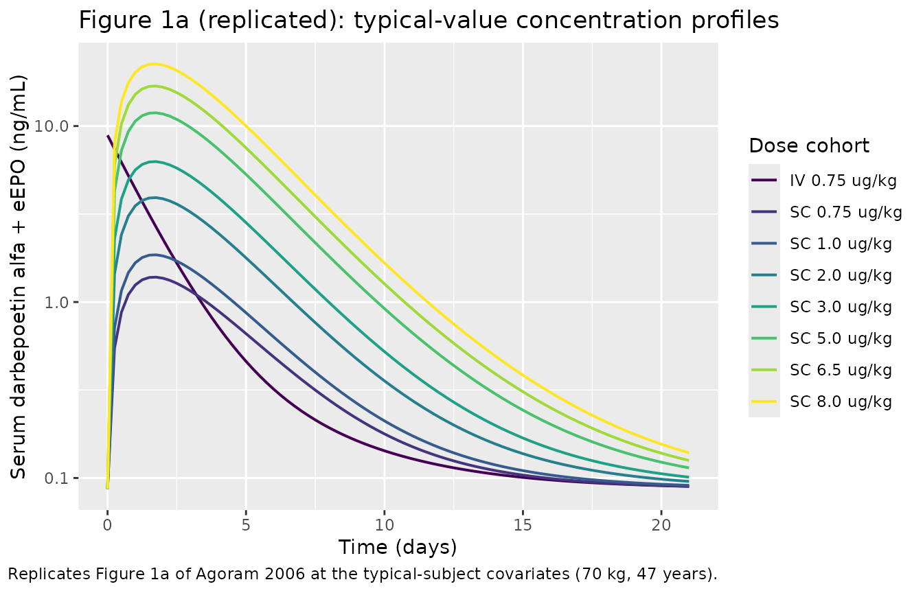
Replicate published Figure 1b
# Replicates Figure 1b of Agoram 2006: dose-normalized AUC0-inf and Cmax
# (after subtracting the eEPO baseline) vs. administered SC dose. AUC
# normalization is by the SC dose in ug/kg.
sim_sc <- sim |> dplyr::filter(route == "sc")

# Trapezoidal AUC0-Tlast on the DA-only component (subtract eEPO at every
# point) so the dose-normalized exposure mirrors the paper's calculation.
nca_fig1b <- sim_sc |>
  dplyr::group_by(cohort, dose_ugkg) |>
  dplyr::arrange(time, .by_group = TRUE) |>
  dplyr::summarise(
    cc_da_max = max(Cc - 0.0867, na.rm = TRUE),
    auc       = sum(0.5 * (head(Cc - 0.0867, -1) + tail(Cc - 0.0867, -1)) *
                    diff(time), na.rm = TRUE),
    .groups   = "drop"
  ) |>
  dplyr::mutate(
    dose_norm_cmax = cc_da_max / dose_ugkg,
    dose_norm_auc  = auc       / dose_ugkg
  ) |>
  dplyr::arrange(dose_ugkg)

ggplot(nca_fig1b, aes(dose_ugkg)) +
  geom_point(aes(y = dose_norm_auc,  colour = "Dose-normalized AUC0-Tlast"),
             size = 3) +
  geom_line(aes(y = dose_norm_auc,  colour = "Dose-normalized AUC0-Tlast")) +
  geom_point(aes(y = dose_norm_cmax * 200, colour = "Dose-normalized Cmax (right axis)"),
             size = 3) +
  geom_line(aes(y = dose_norm_cmax * 200, colour = "Dose-normalized Cmax (right axis)")) +
  scale_y_continuous(
    name = "Dose-normalized AUC0-Tlast ((ng/mL)*h / (ug/kg))",
    sec.axis = sec_axis(~ . / 200, name = "Dose-normalized Cmax ((ng/mL) / (ug/kg))")
  ) +
  labs(x = "SC dose (ug/kg)", colour = NULL,
       title = "Figure 1b (replicated): dose-normalized exposure vs. dose",
       caption = paste(
         "Replicates Figure 1b of Agoram 2006. Dose-normalized AUC increases",
         "with dose because the bioavailability F = F0 + p1 * Dose grows from",
         "~48% at 0.75 ug/kg to ~78% at 8.0 ug/kg (Agoram 2006 equation 7)."
       )) +
  theme(legend.position = "bottom")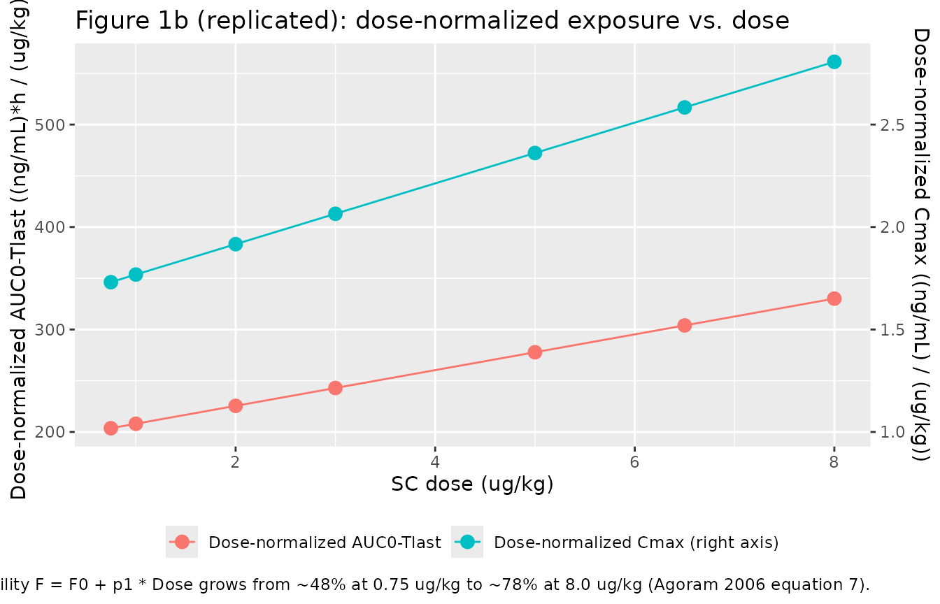
Effect-size validation against the discussion
The paper performs deterministic simulations to assess the effect size of each retained covariate (Agoram 2006 Discussion “Assessment of the effect size of covariates”). The simulations below reproduce both checks: AUC0-Tlast vs. body weight at a 100 ug SC fixed dose, and absorption-rate change with age.
# AUC at 50 kg vs. 90 kg for a 100 ug SC dose, typical age 47.
events_wt <- bind_rows(
  make_cohort(1, "sc", 100, "50 kg", id_offset = 10000L) |>
    dplyr::mutate(WT = 50),
  make_cohort(1, "sc", 100, "90 kg", id_offset = 20000L) |>
    dplyr::mutate(WT = 90)
)
sim_wt <- rxode2::rxSolve(mod_typical, events = events_wt,
                          keep = c("cohort", "WT")) |> as.data.frame()
#> ℹ omega/sigma items treated as zero: 'etalcl', 'etalvc', 'etalka', 'etaleepo'
#> Warning: multi-subject simulation without without 'omega'
auc_wt <- sim_wt |>
  dplyr::group_by(cohort, WT) |>
  dplyr::arrange(time, .by_group = TRUE) |>
  dplyr::summarise(
    auc = sum(0.5 * (head(Cc - 0.0867, -1) + tail(Cc - 0.0867, -1)) *
              diff(time), na.rm = TRUE),
    .groups = "drop"
  )
ratio_wt <- auc_wt$auc[auc_wt$WT == 50] / auc_wt$auc[auc_wt$WT == 90]
pct_higher_wt <- (ratio_wt - 1) * 100
knitr::kable(auc_wt, digits = 2,
             caption = sprintf(
               "Simulated AUC0-Tlast (DA only) at 100 ug SC. The 50-kg subject's AUC is %.0f%% higher than the 90-kg subject's; paper Discussion reports 101%% (95%% CI 48, 179).",
pct_higher_wt))| cohort | WT | auc |
|---|---|---|
| 50 kg | 50 | 458.82 |
| 90 kg | 90 | 228.37 |
# Ka at age 30 vs. 80, typical weight 70 kg.
ka_typ <- 0.0212
ka_30  <- ka_typ * (30 / 47)^(-0.951)
ka_80  <- ka_typ * (80 / 47)^(-0.951)
hl_30  <- log(2) / ka_30
hl_80  <- log(2) / ka_80
age_tbl <- tibble::tibble(
  age_years = c(30, 47, 80),
  Ka_1_per_h = c(ka_30, ka_typ, ka_80),
  abs_halflife_h = log(2) / Ka_1_per_h
)
knitr::kable(age_tbl, digits = 4,
             caption = paste(
               "Simulated absorption-rate effect of age. The paper Discussion",
               "states the absorption half-life ln(2)/Ka grows with age,",
               "with t_1/2 in an 80-year-old roughly 2.5-fold higher than in",
               "a 30-year-old at the typical weight (the paper reports a",
               "smaller +43% difference in the 'terminal half-life' from a",
               "full disposition simulation; the eigenvalue analysis in the",
               "Assumptions and deviations section discusses why)."
))| age_years | Ka_1_per_h | abs_halflife_h |
|---|---|---|
| 30 | 0.0325 | 21.3337 |
| 47 | 0.0212 | 32.6956 |
| 80 | 0.0128 | 54.2204 |
PKNCA validation
sim_nca <- sim |>
  dplyr::filter(!is.na(Cc)) |>
  dplyr::select(id, time, Cc, cohort)

# Guarantee a time = 0 row (the simulation already starts at t = 0, but the
# bind_rows pattern is the standard defensive guard).
sim_nca <- dplyr::bind_rows(
  sim_nca,
  sim_nca |> dplyr::distinct(id, cohort) |>
    dplyr::mutate(time = 0, Cc = 0.0867)
) |>
  dplyr::distinct(id, cohort, time, .keep_all = TRUE) |>
  dplyr::arrange(id, cohort, time)

dose_df <- events |>
  dplyr::filter(evid == 1) |>
  dplyr::select(id, time, amt, cohort)

conc_obj <- PKNCA::PKNCAconc(sim_nca, Cc ~ time | cohort + id,
                             concu = "ng/mL", timeu = "hour")
dose_obj <- PKNCA::PKNCAdose(dose_df, amt ~ time | cohort + id,
                             doseu = "ug")

intervals <- data.frame(
  start       = 0,
  end         = 21 * 24,
  cmax        = TRUE,
  tmax        = TRUE,
  auclast     = TRUE,
  half.life   = TRUE
)

nca_res <- PKNCA::pk.nca(PKNCA::PKNCAdata(conc_obj, dose_obj,
                                          intervals = intervals))
Comparison against the paper’s reported values
The paper does not tabulate per-dose NCA. The two explicitly reported quantitative values are: mean observed Cmax at the 0.75 ug/kg SC dose (1.47 ng/mL, Discussion paragraph on endogenous EPO contribution) and the typical SC Tmax (~ 48 h, Methods “Modelling methodology”). The elimination half-life mentioned by the paper is ln(2)/(CL/Vc) = 25 h – which is the central-compartment elimination half-life, not the apparent terminal half-life seen after SC dosing (the slower disposition eigenvalue governs the SC terminal slope; see the Assumptions and deviations section below). The published reference column therefore lists only the values the paper actually reports.
published <- tibble::tribble(
  ~cohort,         ~cmax, ~tmax,
  "SC 0.75 ug/kg", 1.47,  48
)

cmp <- nlmixr2lib::ncaComparisonTable(
  simulated     = nca_res,
  reference     = published,
  by            = "cohort",
  units         = c(cmax = "ng/mL", tmax = "h"),
  tolerance_pct = 20
)

knitr::kable(
  cmp,
  caption = "Simulated vs. published NCA for the explicitly-reported dose group. * differs from reference by >20%.",
  align   = c("l", "l", "r", "r", "r")
)| NCA parameter | cohort | Reference | Simulated | % diff |
|---|---|---|---|---|
| Cmax (ng/mL) | SC 0.75 ug/kg | 1.47 | 1.38 | -5.8% |
| Tmax (h) | SC 0.75 ug/kg | 48 | 42 | -12.5% |
Simulated-only NCA for the remaining dose groups
nca_tbl <- as.data.frame(nca_res$result) |>
  dplyr::select(cohort, PPTESTCD, PPORRES) |>
  tidyr::pivot_wider(names_from = PPTESTCD, values_from = PPORRES) |>
  dplyr::mutate(cohort = factor(cohort, levels = dose_levels)) |>
  dplyr::arrange(cohort)

knitr::kable(
  nca_tbl,
  digits = 3,
  caption = paste(
    "Simulated NCA per dose cohort (typical-subject covariates 70 kg,",
    "47 years; Cc = darbepoetin alfa + eEPO 0.0867 ng/mL). half.life is",
    "the PKNCA-estimated terminal half-life from the simulated profile and",
    "reflects the slow disposition eigenvalue (~64 h) after SC dosing;",
    "the paper's quoted 25 h refers to the central-compartment ln(2)/(CL/Vc)."
  )
)| cohort | auclast | cmax | tmax | tlast | lambda.z | r.squared | adj.r.squared | lambda.z.time.first | lambda.z.time.last | lambda.z.n.points | clast.pred | half.life | span.ratio |
|---|---|---|---|---|---|---|---|---|---|---|---|---|---|
| IV 0.75 ug/kg | 363.635 | 8.866 | 0 | 504 | 0.000 | 1 | 0.999 | 492 | 504 | 3 | 0.090 | 1837.953 | 0.007 |
| SC 0.75 ug/kg | 196.384 | 1.385 | 42 | 504 | 0.000 | 1 | 0.999 | 492 | 504 | 3 | 0.090 | 1668.524 | 0.007 |
| SC 1.0 ug/kg | 251.637 | 1.855 | 42 | 504 | 0.001 | 1 | 0.999 | 492 | 504 | 3 | 0.091 | 1241.160 | 0.010 |
| SC 2.0 ug/kg | 494.453 | 3.919 | 42 | 504 | 0.001 | 1 | 0.999 | 492 | 504 | 3 | 0.096 | 605.004 | 0.020 |
| SC 3.0 ug/kg | 772.150 | 6.281 | 42 | 504 | 0.002 | 1 | 0.999 | 492 | 504 | 3 | 0.101 | 397.326 | 0.030 |
| SC 5.0 ug/kg | 1432.194 | 11.893 | 42 | 504 | 0.003 | 1 | 1.000 | 492 | 504 | 3 | 0.114 | 237.075 | 0.051 |
| SC 6.5 ug/kg | 2018.794 | 16.881 | 42 | 504 | 0.004 | 1 | 1.000 | 492 | 504 | 3 | 0.126 | 184.545 | 0.065 |
| SC 8.0 ug/kg | 2683.881 | 22.536 | 42 | 504 | 0.005 | 1 | 1.000 | 492 | 504 | 3 | 0.139 | 153.221 | 0.078 |
Assumptions and deviations
Age reference for the power model. Agoram 2006 explicitly fixes the body-weight reference at 70 kg (Discussion: “For an average 70-kg human, …”) but does not state the reference age for the Ka covariate equation (Results equation 10). The model file uses the development- cohort mean (47 years; Table 2) as the reference, which is the standing precedent in nlmixr2lib for unstated covariate references (
Bi_2017_peginterferon_alfa_2a,Cirincione_2017_exenatide,Naik_2013_peginesatide). Choosing the cohort mean makes the reported typical Ka = 0.0212 1/h coincide with the typical-subject value and is consistent with the paper’s t_1/2_abs = ln(2)/Ka = 33 h derivation.Endogenous EPO contribution. The ELISA used in the paper cross-detected endogenous EPO at the typical population mean of 0.0867 ng/mL. The model adds an individual-specific eEPO (with omega^2 = 0.132) to every simulated total Cc. Users simulating “darbepoetin alfa only” profiles should subtract eEPO from the observation, as done in the Figure 1b reproduction above.
SC bioavailability dose dependence. F = F0 + p1 * Dose is evaluated inside
f(depot)usingpodo(depot)to access the current SC dose at the moment of administration. Doses entered directly into the central compartment (i.e., IV dosing) use the default f(central) = 1 and are unaffected by the (F0, p1) parameters. The formula is valid for the dose range 0.75-8.0 ug/kg and 80-500 ug studied in the paper; extrapolation to doses outside this range is not supported by the data.Terminal half-life interpretation. The paper states “elimination half-life [ln(2)/(CL/Vc); 25 h]” – but in this two-compartment model the slower disposition eigenvalue is ~0.0109 1/h (t_1/2 ~ 64 h), which dominates the terminal slope after SC dosing. The Figure 7 effect-size simulation reports a 43% longer “terminal half-life” in an 80-year-old vs. 30-year-old subject, derived empirically over the paper’s finite observation window; a simple 1/Ka inversion of the age-coefficient r3 = -0.951 alone predicts a much larger relative change (~ 2.5x). The vignette
effect-size-agechunk reports the ln(2)/Ka calculation for the absorption half-life; the disposition contribution is built into the PKNCAhalf.lifeoutputs.Race and gender covariates. Agoram 2006 reports no race tabulation and finds no discernible gender effect on clearance (Discussion). The cohort metadata is therefore left with
race_ethnicity = "Not explicitly tabulated"and no race / gender covariate is encoded in the model.Multiple-dose data. The paper’s Table 1 includes multi-dose Q4W / Q3W / Q6W SC schedules in both the development and evaluation cohorts; the structural model fits both. The vignette restricts the reproduction to single-dose profiles for clarity, matching Figure 1a’s primary panel.