Metformin + cimetidine renal transporter interaction (Nishiyama 2019)
Source:vignettes/articles/Nishiyama_2019_metformin_cimetidine.Rmd
Nishiyama_2019_metformin_cimetidine.RmdModel and source
This paper contributes three model files, because the authors built three models: a metformin PBPK model, a cimetidine PBPK model, and the combined system in which cimetidine competitively inhibits metformin’s transporters.
Nishiyama_2019_metformin_pbpk– metformin alone (53 ODE states)Nishiyama_2019_cimetidine_pbpk– cimetidine alone (27 ODE states)Nishiyama_2019_metformin_cimetidine_ddi_pbpk– both together (80 ODE states)Citation: Nishiyama K, Toshimoto K, Lee W, Ishiguro N, Bister B, Sugiyama Y. Physiologically-Based Pharmacokinetic Modeling Analysis for Quantitative Prediction of Renal Transporter-Mediated Interactions Between Metformin and Cimetidine. CPT Pharmacometrics Syst Pharmacol. 2019;8(6):396-406. doi:10.1002/psp4.12398. Erratum: CPT Pharmacometrics Syst Pharmacol. 2020;9:606-608. doi:10.1002/psp4.12539. The ODE system and the hybrid-to-elementary parameter conversions are transcribed from Supplementary Material S2 (‘Model equations for metformin’, file PSP4-8-396-s008.pdf) and the Supplemental Text (PSP4-8-396-s007.pdf). Drug parameters are Table S1 (PSP4-8-396-s003.pdf), body physiology is Table S2 (PSP4-8-396-s004.pdf) and kidney physiology is Table S3 (PSP4-8-396-s005.pdf). Fitted ka, ktrans and RMATE/dif are Table 1 of the article. See the vignette Errata for the transcription corrections applied to the published equation list.
Article: https://doi.org/10.1002/psp4.12398
Erratum: Nishiyama K et al. CPT Pharmacometrics Syst Pharmacol. 2020;9:606-608, https://doi.org/10.1002/psp4.12539 (PMC7577014). It changes one equation of the metformin liver and corrects the Supplementary Material S2 equation list; see Published erratum for what it means for these models.
Supplements (open access, same DOI): Tables S1-S4 and the two supplemental model documents
PSP4-8-396-s003.pdfthroughPSP4-8-396-s008.pdf.
All three models carry their amounts in micrograms and their
concentrations in ug/L, with every volume in litres, so a dose in
milligrams is entered as amt = <mg> * 1000.
met <- rxode2::rxode2(readModelDb("Nishiyama_2019_metformin_pbpk"))
cim <- rxode2::rxode2(readModelDb("Nishiyama_2019_cimetidine_pbpk"))
ddi <- rxode2::rxode2(readModelDb("Nishiyama_2019_metformin_cimetidine_ddi_pbpk"))
c(metformin = length(met$state), cimetidine = length(cim$state), ddi = length(ddi$state))
#>  metformin cimetidine        ddi
#>         53         27         80
What the paper is about
Metformin is cleared almost entirely by the kidney, and its renal clearance exceeds the glomerular filtration rate, so it is actively secreted: taken up across the basolateral membrane of the proximal tubule by OCT2 and pumped into the urine across the luminal membrane by MATE1 and MATE2-K. Cimetidine inhibits both, and raises metformin exposure about 50% in healthy volunteers.
The problem the paper addresses is that the previously published PBPK models could only reproduce that interaction after lowering cimetidine’s inhibition constants far below their measured in vitro values – by roughly 500-fold for the conventional model and 8- to 18-fold for the “electrochemical” model. A model that needs its inhibition constants retuned per interaction cannot be used to predict a new one.
The authors’ change is small and specific: OCT1 and OCT2 are electrogenic, so their transport is driven by the membrane potential, and the earlier model let that potential move with the metformin concentration. Here it is held constant, on the argument that the membrane potential is set by ions present at 100-200 mmol/L and is not perturbed measurably by a drug at micromolar concentrations. With that one change the interaction is reproduced using in vitro inhibition constants, and the sensitivity analysis then identifies MATE inhibition – not OCT2 inhibition – as the mechanism.
Population
These are not population models fitted to individual-level data. The physiology is the standard 70 kg adult of Davies & Morris 1993 (Table S2), with the kidney geometry of Table S3, and the models were fitted to, or compared against, published mean profiles from three studies:
-
Metformin 1,500 mg single oral dose – plasma and
whole-blood concentrations and urinary excretion, Tucker et al. 1981 (Br
J Clin Pharmacol 12:235-246). This is the data set that determined
ka,ktransandRMATE/dif. -
Metformin 250 mg single oral dose, with and without 400 mg
cimetidine – the six-subject crossover of Somogyi et al. 1987
(Br J Clin Pharmacol 23:545-551), which supplies both the control arm
used to re-fit
ktransandRMATE/difat 250 mg and the observed interaction ratios. - Cimetidine 400 mg single oral dose – Grahnen et al. 1979 (Eur J Clin Pharmacol 16:335-340).
str(readModelDb("Nishiyama_2019_metformin_cimetidine_ddi_pbpk")()$population)
#> List of 5
#>  $ species      : chr "human"
#>  $ n_subjects   : int 6
#>  $ disease_state: chr "healthy adults"
#>  $ dose_range   : chr "250 mg metformin with and without 400 mg cimetidine, single oral doses"
#>  $ notes        : chr "The interaction reproduced is the six-subject crossover of Somogyi et al. 1987 (Br J Clin Pharmacol 23:545-551)"| __truncated__
Source trace
Every ini() entry in the three model files carries an
in-file comment naming its source table. The table below collects the
structural equations and the parameters that are not simply
physiology.
| Equation / parameter | Value | Source location |
|---|---|---|
Erythrocyte partitioning, kin_rbc /
kout_rbc
|
0.006 / 0.02 per h | Methods eqs. 1-2; Table S1 |
| OCT1 bidirectional transport | Michaelis-Menten with exp(N_h) / R_OCT1,inf/eff
|
Methods eq. 3-4 |
| OCT2 bidirectional transport | Michaelis-Menten with exp(N_vpt) / R_OCT2,inf/eff
|
Methods eq. 5 |
| MATE efflux | Michaelis-Menten, Vmax,MATE / (Km,MATE + C_cell)
|
Methods eq. 6 |
CL_int,sec = PS_r,inf * beta_kidney |
– | Methods eqs. 7-14 |
Competitive inhibition
PS_act(+I) = PS_act / (1 + I/Ki)
|
– | Methods eq. 15 |
| Hepatic hybrid-to-elementary conversion | PS_h,act = CL_int,all / (beta_liver (1 + R_dif)) |
Supplemental Text eqs. 1-5; Suppl. S2 “Other equations” |
Hepatic CL_int,met
|
CL_int,all / ((1 - beta_liver)(1 + R_dif)) * R_dif / gamma_h |
Erratum eq. 1 – the form the authors ran; see Published erratum |
Nernst ratio gamma_h
|
4.46 | Supplemental Text eq. 7 |
Metformin ka
|
0.21 /h | Table 1 (both dose panels) |
Metformin ktrans
|
2.4 /h (1,500 mg); 0.61 /h (250 mg) | Table 1 |
Metformin RMATE/dif
|
153 / 213 / 325 / 814 (1,500 mg); 183 / 261 / 402 / 1,143 (250 mg) | Table 1 |
Metformin FaFg
|
0.57 (1,500 mg); 0.84 (250 mg) | Table S1 |
Metformin CL_int,all, R_dif,
beta_liver
|
10.7 L/h, 0.186, 0.5 | Table S1 |
Metformin Kp adipose / muscle / skin |
0.27 / 2.09 / 1.46 | Table S1 |
Metformin in vitro Km OCT1 / OCT2 / MATEs |
1,470 / 1,178 / 740 umol/L | Table S1 |
Metformin Pd, membrane potential |
1.8e-5 m/h, -40 mV (liver) | Table S1 |
| Body volumes and blood flows | – | Table S2 |
| Kidney flows, areas, potentials, pH | – | Table S3 |
| Cimetidine compound layer | – | Table S4 |
Cimetidine Ki OCT1 / OCT2 / MATEs |
104 / 159 / 3.93 umol/L | Table 2 footnote |
Fitted in vivo Ki for MATEs |
1.71 / 1.34 / 0.64 / 0.23 umol/L | Table 3 (pre-erratum; the erratum’s recalculated range is 0.25-1.2
umol/L, not printed per beta_kidney) |
Structural check: mass balance
Before comparing any number to the paper, check the topology. Each
model carries explicit sinks (a_feces,
a_metab, urine) alongside every distribution
state, so the sum over all states must equal the dose
at all times. A missing, duplicated or mis-signed flow term in an
80-state transcription of a PDF equation list is invisible to inspection
but shows up here immediately.
total_mass <- function(mod, ev, dose_ug, states) {
  s <- as.data.frame(rxode2::rxSolve(mod, ev, atol = 1e-9, rtol = 1e-9, addDosing = FALSE))
  rowSums(s[, states, drop = FALSE]) / dose_ug
}

# The observation grid starts at 1 h, after cimetidine's 0.15 h absorption lag.
# During the lag the dose is genuinely in no compartment -- rxode2 holds it
# outside the system until t = tlag -- so a t = 0 record would report zero mass
# for a reason that has nothing to do with the topology being checked.
mb_grid <- seq(1, 24, by = 1)
ev_met <- rxode2::et(amt = 1500 * 1000, cmt = "transit1") |> rxode2::et(mb_grid)
ev_cim <- rxode2::et(amt = 400 * 1000, cmt = "intestine") |> rxode2::et(mb_grid)
ev_ddi <- rxode2::et(amt = 250 * 1000, cmt = "transit1_met") |>
  rxode2::et(amt = 400 * 1000, cmt = "intestine_cim") |>
  rxode2::et(mb_grid)

mb_met <- total_mass(met, ev_met, 1500 * 1000, met$state)
mb_cim <- total_mass(cim, ev_cim, 400 * 1000, cim$state)
mb_ddi_met <- total_mass(ddi, ev_ddi, 250 * 1000, grep("_met$", ddi$state, value = TRUE))
mb_ddi_cim <- total_mass(ddi, ev_ddi, 400 * 1000, grep("_cim$", ddi$state, value = TRUE))

data.frame(
  model = c("metformin", "cimetidine", "DDI (metformin states)", "DDI (cimetidine states)"),
  worst_relative_error = c(
    max(abs(mb_met - 1)), max(abs(mb_cim - 1)),
    max(abs(mb_ddi_met - 1)), max(abs(mb_ddi_cim - 1))
  )
)
#>                     model worst_relative_error
#> 1               metformin         1.776357e-15
#> 2              cimetidine         1.554312e-15
#> 3  DDI (metformin states)         8.881784e-16
#> 4 DDI (cimetidine states)         3.885781e-15

# The two sides of the interaction model must conserve their own drug
# independently -- cimetidine inhibits metformin's carriers but no mass
# crosses between the two systems.
stopifnot(
  max(abs(mb_met - 1)) < 1e-6,
  max(abs(mb_cim - 1)) < 1e-6,
  max(abs(mb_ddi_met - 1)) < 1e-6,
  max(abs(mb_ddi_cim - 1)) < 1e-6
)
Derived-parameter check
The paper’s Discussion prints the elementary renal parameters it
back-solves from beta_kidney and RMATE/dif for
the 1,500 mg fit at beta_kidney = 0.1. Those are a direct,
deterministic check on the hybrid-to-elementary conversion before any
ODE is integrated: they involve no data, no integration and no fitting,
so they either reproduce or the transcription is wrong.
d <- as.data.frame(rxode2::rxSolve(
  met, rxode2::et(amt = 1, cmt = "transit1") |> rxode2::et(0),
  atol = 1e-9, rtol = 1e-9, addDosing = FALSE
))[1, ]

derived <- data.frame(
  quantity = c(
    "PS_OCT2,inf (L/h)", "PS_MATE (L/h)", "PS_r,dif,inf (L/h)",
    "PS_r,dif,eff (L/h)", "exp(N)/R_OCT2,inf/eff", "gamma_h"
  ),
  paper = c(732, 4.47, 0.043, 0.0031, 0.055, 4.46),
  model = c(
    d$ps_oct2, d$ps_mate, d$ps_r_pt_difinf, d$ps_r_pt_difeff,
    d$envpt / 1.32, d$gamma_h
  )
)
derived$pct_diff <- 100 * (derived$model - derived$paper) / derived$paper
knitr::kable(derived, digits = c(0, 4, 4, 1))| quantity | paper | model | pct_diff |
|---|---|---|---|
| PS_OCT2,inf (L/h) | 732.0000 | 733.6630 | 0.2 |
| PS_MATE (L/h) | 4.4700 | 4.4649 | -0.1 |
| PS_r,dif,inf (L/h) | 0.0430 | 0.0412 | -4.2 |
| PS_r,dif,eff (L/h) | 0.0031 | 0.0030 | -3.3 |
| exp(N)/R_OCT2,inf/eff | 0.0550 | 0.0551 | 0.2 |
| gamma_h | 4.4600 | 4.4702 | 0.2 |
PS_OCT2,inf, PS_MATE, the electrochemical
factor and gamma_h reproduce to better than 1%, which
confirms the whole extended-clearance chain – eq. 7 through eq. 14 plus
the Nernst terms – was transcribed correctly. The two passive-diffusion
terms sit about 4% high; they are printed to two significant figures in
a Discussion worked example, and because the paper’s own
PS_OCT2,inf is reproduced using this model’s
PS_u,PT,dif,eff rather than the rounded one it prints, the
rounding is in the printed value rather than in the transcription. See
Errata.
Metformin alone
Figure 2a-d: 1,500 mg single oral dose
The whole point of the erythrocyte compartments is the slow rise of
the blood-to-plasma ratio, which the model reproduces as a structural
consequence of kin_rbc << kout_rbc being
slow relative to distribution rather than as a fitted time-varying
parameter.
grid_fine <- seq(0, 24, by = 0.05)
s1500 <- as.data.frame(rxode2::rxSolve(
  met,
  rxode2::et(amt = 1500 * 1000, cmt = "transit1") |> rxode2::et(grid_fine),
  atol = 1e-9, rtol = 1e-9, addDosing = FALSE
))

s1500 |>
  dplyr::select(time, Plasma = Cc, Blood = Cb) |>
  tidyr::pivot_longer(-time, names_to = "matrix", values_to = "conc") |>
  ggplot2::ggplot(ggplot2::aes(time, conc, colour = matrix)) +
  ggplot2::geom_line(linewidth = 0.8) +
  ggplot2::labs(
    x = "Time (h)", y = "Metformin concentration (ug/L)", colour = NULL,
    title = "Replicates Figure 2a-d of Nishiyama 2019 (1,500 mg oral)"
  ) +
  ggplot2::theme_bw()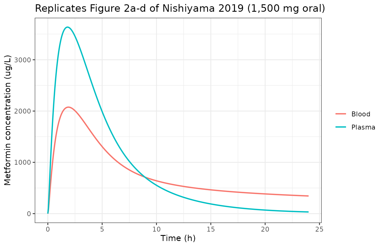
ggplot2::ggplot(s1500, ggplot2::aes(time, Cb / Cc)) +
  ggplot2::geom_line(linewidth = 0.8) +
  ggplot2::labs(
    x = "Time (h)", y = "Blood-to-plasma ratio",
    title = "Blood-to-plasma ratio rises with time (Figure 2d)"
  ) +
  ggplot2::theme_bw()
#> Warning: Removed 1 row containing missing values or values outside the scale range
#> (`geom_line()`).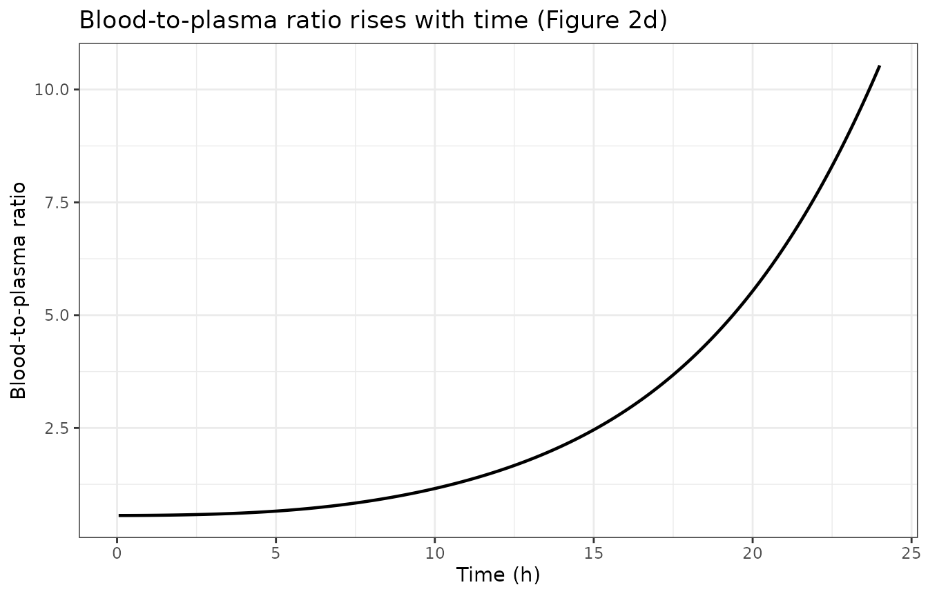
ggplot2::ggplot(s1500, ggplot2::aes(time, urine / 1000)) +
  ggplot2::geom_line(linewidth = 0.8) +
  ggplot2::labs(
    x = "Time (h)", y = "Cumulative urinary metformin (mg)",
    title = "Replicates Figure S1 of Nishiyama 2019 (1,500 mg oral)"
  ) +
  ggplot2::theme_bw()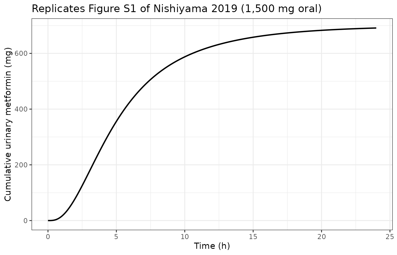
Figure 2e-h: 250 mg single oral dose
The 250 mg absorption parameters differ (ktrans 0.61 /h,
FaFg 0.84), and RMATE/dif was re-fitted at
183. Overriding them on the shipped model is how a user switches dose
level.
pars250 <- c(lktrans = log(0.61), fafg = 0.84, lr_mate_dif = log(183))
s250 <- as.data.frame(rxode2::rxSolve(
  met,
  rxode2::et(amt = 250 * 1000, cmt = "transit1") |> rxode2::et(seq(0, 12, by = 0.05)),
  params = pars250, atol = 1e-9, rtol = 1e-9, addDosing = FALSE
))

ggplot2::ggplot(s250, ggplot2::aes(time, Cc)) +
  ggplot2::geom_line(linewidth = 0.8) +
  ggplot2::labs(
    x = "Time (h)", y = "Metformin plasma concentration (ug/L)",
    title = "Replicates Figure 2e-h of Nishiyama 2019 (250 mg oral)"
  ) +
  ggplot2::theme_bw()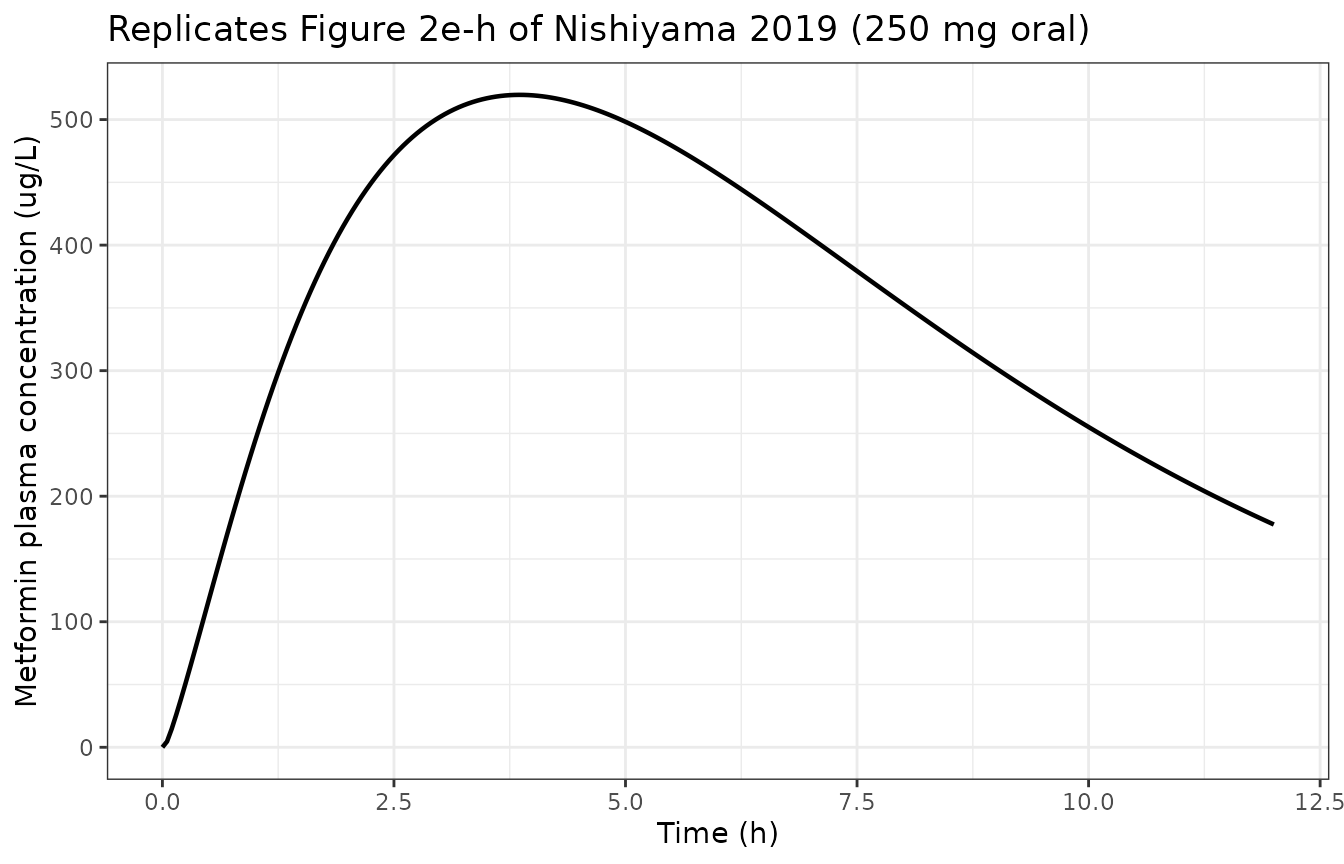
Cimetidine, Figure 2i
scim <- as.data.frame(rxode2::rxSolve(
  cim,
  rxode2::et(amt = 400 * 1000, cmt = "intestine") |> rxode2::et(seq(0, 24, by = 0.02)),
  atol = 1e-9, rtol = 1e-9, addDosing = FALSE
))

ggplot2::ggplot(scim, ggplot2::aes(time, Cc)) +
  ggplot2::geom_line(linewidth = 0.8) +
  ggplot2::labs(
    x = "Time (h)", y = "Cimetidine plasma concentration (ug/L)",
    title = "Replicates Figure 2i of Nishiyama 2019 (400 mg oral)"
  ) +
  ggplot2::theme_bw()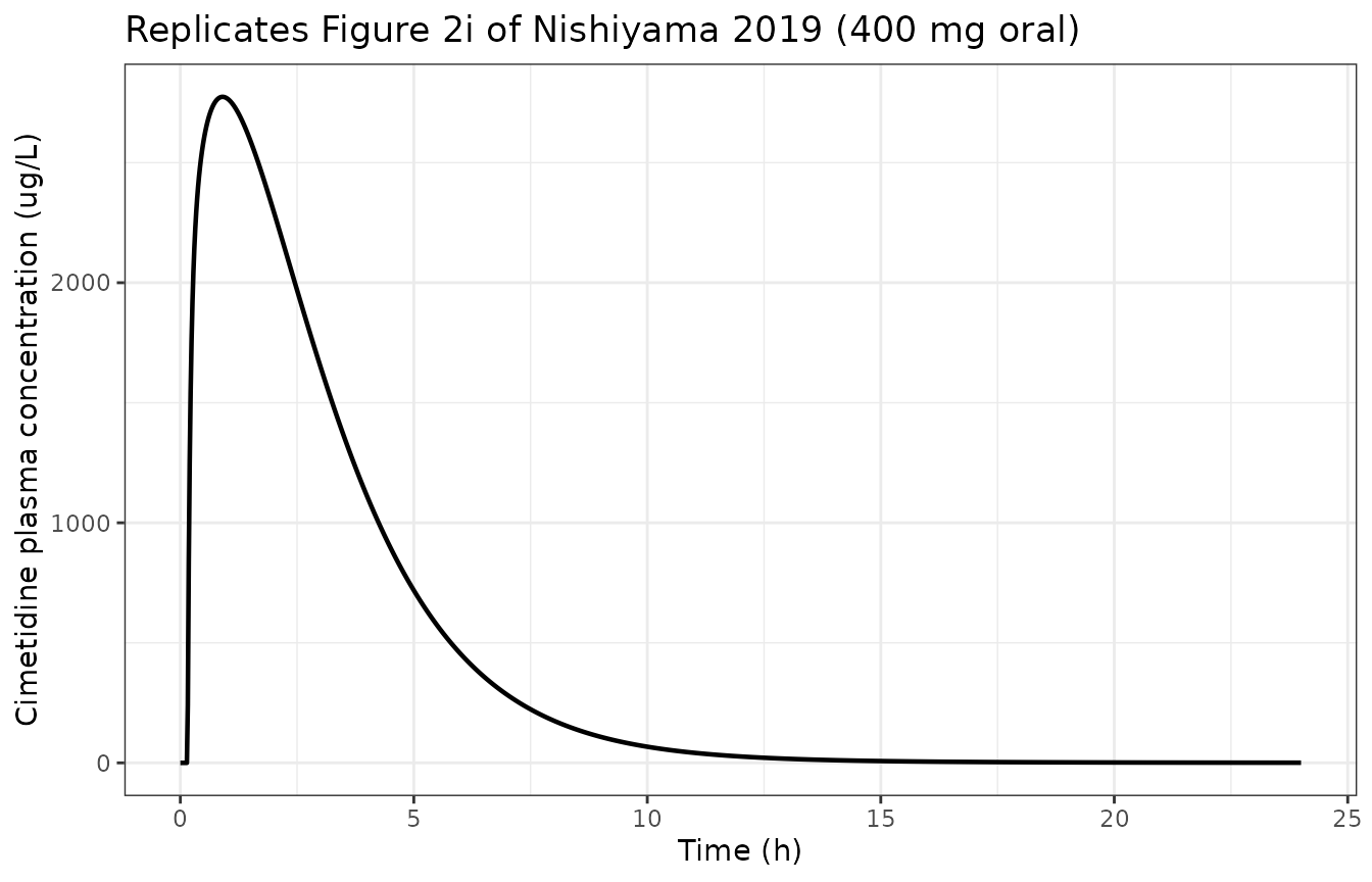
NCA validation with PKNCA
conc_data <- dplyr::bind_rows(
  s1500 |> dplyr::transmute(id = 1L, treatment = "Metformin 1,500 mg", time, Cc),
  s250 |> dplyr::transmute(id = 1L, treatment = "Metformin 250 mg", time, Cc),
  scim |> dplyr::transmute(id = 1L, treatment = "Cimetidine 400 mg", time, Cc)
) |>
  dplyr::filter(!is.na(Cc))

dose_data <- data.frame(
  id = 1L,
  treatment = c("Metformin 1,500 mg", "Metformin 250 mg", "Cimetidine 400 mg"),
  amt = c(1500, 250, 400),
  time = 0
)

intervals <- data.frame(
  treatment = c("Metformin 1,500 mg", "Metformin 250 mg", "Cimetidine 400 mg"),
  start = 0,
  end = c(24, 12, 24),
  cmax = TRUE, tmax = TRUE, auclast = TRUE
)

o_conc <- PKNCA::PKNCAconc(conc_data, Cc ~ time | id / treatment)
o_dose <- PKNCA::PKNCAdose(dose_data, amt ~ time | id + treatment)
o_data <- PKNCA::PKNCAdata(o_conc, o_dose, intervals = intervals)
res <- PKNCA::pk.nca(o_data)
knitr::kable(
  as.data.frame(res) |>
    dplyr::select(treatment, PPTESTCD, PPORRES) |>
    dplyr::mutate(PPORRES = signif(PPORRES, 4)),
  caption = "PKNCA non-compartmental parameters from the simulated profiles"
)| treatment | PPTESTCD | PPORRES |
|---|---|---|
| Metformin 1,500 mg | auclast | 21920.00 |
| Metformin 1,500 mg | cmax | 3636.00 |
| Metformin 1,500 mg | tmax | 1.80 |
| Metformin 250 mg | auclast | 4277.00 |
| Metformin 250 mg | cmax | 519.70 |
| Metformin 250 mg | tmax | 3.85 |
| Cimetidine 400 mg | auclast | 10420.00 |
| Cimetidine 400 mg | cmax | 2774.00 |
| Cimetidine 400 mg | tmax | 0.90 |
Comparison against the published simulated and observed values
Table 1 of the paper reports both the observed summary statistics and the values its own simulation produced, and the simulated values are the correct comparator for a transcription check: the observed values carry the between-subject spread of the original studies, whereas the paper’s simulated values are what a correct transcription of the same equations and parameters must return.
reference <- data.frame(
  treatment = c("Metformin 1,500 mg", "Metformin 250 mg", "Cimetidine 400 mg"),
  # Table 1, 1,500 mg panel: AUC0-24 20.1 mg*h/L at beta_kidney 0.1
  # Table 1, 250 mg panel: AUC0-12 4.12 mg*h/L, Cmax 502 ug/L, Tmax 3.72 h
  # Results, cimetidine PBPK model: simulated AUC 9.10 mg*h/L
  auclast = c(20.1, 4.12, 9.10) * 1000,
  cmax = c(NA, 502, NA),
  tmax = c(NA, 3.72, NA)
)

tbl <- nlmixr2lib::ncaComparisonTable(
  res, reference,
  by = "treatment",
  units = c(cmax = "ug/L", auclast = "ug*h/L", tmax = "h")
)
knitr::kable(tbl, caption = "Simulated vs. the paper's own simulated values")| NCA parameter | treatment | Reference | Simulated | % diff |
|---|---|---|---|---|
| Cmax (ug/L) | Metformin 1,500 mg | — | 3640 | — |
| Cmax (ug/L) | Metformin 250 mg | 502 | 520 | +3.5% |
| Cmax (ug/L) | Cimetidine 400 mg | — | 2770 | — |
| Tmax (h) | Metformin 1,500 mg | — | 1.8 | — |
| Tmax (h) | Metformin 250 mg | 3.72 | 3.85 | +3.5% |
| Tmax (h) | Cimetidine 400 mg | — | 0.9 | — |
| AUClast (ug*h/L) | Metformin 1,500 mg | 20100 | 21900 | +9.1% |
| AUClast (ug*h/L) | Metformin 250 mg | 4120 | 4280 | +3.8% |
| AUClast (ug*h/L) | Cimetidine 400 mg | 9100 | 10400 | +14.5% |
attr(tbl, "footnote")
#> NULL
Renal clearance is not an NCA parameter PKNCA returns from plasma
alone, so it is checked separately against the urine
state.
auc_of <- function(s, tmax) {
  s <- s[s$time <= tmax, ]
  sum(diff(s$time) * (utils::head(s$Cc, -1) + utils::tail(s$Cc, -1)) / 2) / 1000
}
clr <- data.frame(
  arm = c("Metformin 1,500 mg", "Metformin 250 mg"),
  paper_simulated = c(29.8, 28.5),
  paper_observed = c(23.0, 31.6),
  model = c(
    max(s1500$urine) / 1000 / auc_of(s1500, 24),
    max(s250$urine) / 1000 / auc_of(s250, 12)
  )
)
clr$pct_diff <- 100 * (clr$model - clr$paper_simulated) / clr$paper_simulated
knitr::kable(clr, digits = 1, caption = "Renal clearance (L/h)")| arm | paper_simulated | paper_observed | model | pct_diff |
|---|---|---|---|---|
| Metformin 1,500 mg | 29.8 | 23.0 | 31.5 | 5.8 |
| Metformin 250 mg | 28.5 | 31.6 | 31.8 | 11.4 |
# ncaComparisonTable() formats every column as text for display, so the gate
# recomputes the percent differences numerically from the PKNCA result rather
# than parsing them back out of the rendered table.
chk <- as.data.frame(res) |>
  dplyr::filter(PPTESTCD %in% c("cmax", "tmax", "auclast")) |>
  dplyr::select(treatment, PPTESTCD, simulated = PPORRES) |>
  dplyr::inner_join(
    reference |>
      tidyr::pivot_longer(-treatment, names_to = "PPTESTCD", values_to = "paper"),
    by = c("treatment", "PPTESTCD")
  ) |>
  dplyr::filter(!is.na(paper)) |>
  dplyr::mutate(pct_diff = 100 * (simulated - paper) / paper)
knitr::kable(chk, digits = 2)| treatment | PPTESTCD | simulated | paper | pct_diff |
|---|---|---|---|---|
| Metformin 1,500 mg | auclast | 21924.17 | 20100.00 | 9.08 |
| Metformin 250 mg | auclast | 4277.00 | 4120.00 | 3.81 |
| Metformin 250 mg | cmax | 519.69 | 502.00 | 3.52 |
| Metformin 250 mg | tmax | 3.85 | 3.72 | 3.49 |
| Cimetidine 400 mg | auclast | 10420.30 | 9100.00 | 14.51 |
# Structural gate. Every model here is deterministic -- no etas, no random
# cohort -- so these comparisons are reproducible bit-for-bit across machines
# and a tight bound is appropriate. 15% is the residual transcription
# uncertainty documented in Errata, not sampling noise.
stopifnot(
  nrow(chk) == 5L,
  max(abs(chk$pct_diff)) < 15,
  max(abs(clr$pct_diff)) < 15
)
The drug-drug interaction
Figure 3: metformin with and without cimetidine
ddi_solve <- function(cim_dose, beta_kidney, r_mate_dif, ki_mate_um) {
  ev <- rxode2::et(amt = 250 * 1000, cmt = "transit1_met")
  if (cim_dose > 0) ev <- rxode2::et(ev, amt = cim_dose * 1000, cmt = "intestine_cim")
  as.data.frame(rxode2::rxSolve(
    ddi, rxode2::et(ev, seq(0, 12, by = 0.02)),
    params = c(
      beta_kidney_met = beta_kidney,
      lr_mate_dif_met = log(r_mate_dif),
      ki_mate_um = ki_mate_um
    ),
    atol = 1e-9, rtol = 1e-9, addDosing = FALSE
  ))
}

ddi_metrics <- function(s) {
  auc <- sum(diff(s$time) * (utils::head(s$Cc, -1) + utils::tail(s$Cc, -1)) / 2) / 1000
  c(auc = auc, cmax = max(s$Cc), clr = max(s$urine_met) / 1000 / auc)
}

ctl <- ddi_solve(0, 0.1, 183, 3.93)
ddi_invivo <- ddi_solve(400, 0.1, 183, 1.71)

dplyr::bind_rows(
  ctl |> dplyr::transmute(time, arm = "Metformin alone", Cc),
  ddi_invivo |> dplyr::transmute(time, arm = "Metformin + cimetidine", Cc)
) |>
  ggplot2::ggplot(ggplot2::aes(time, Cc, colour = arm)) +
  ggplot2::geom_line(linewidth = 0.8) +
  ggplot2::labs(
    x = "Time (h)", y = "Metformin plasma concentration (ug/L)", colour = NULL,
    title = "Replicates Figure 3a of Nishiyama 2019 (beta_kidney 0.1, fitted in vivo Ki)"
  ) +
  ggplot2::theme_bw()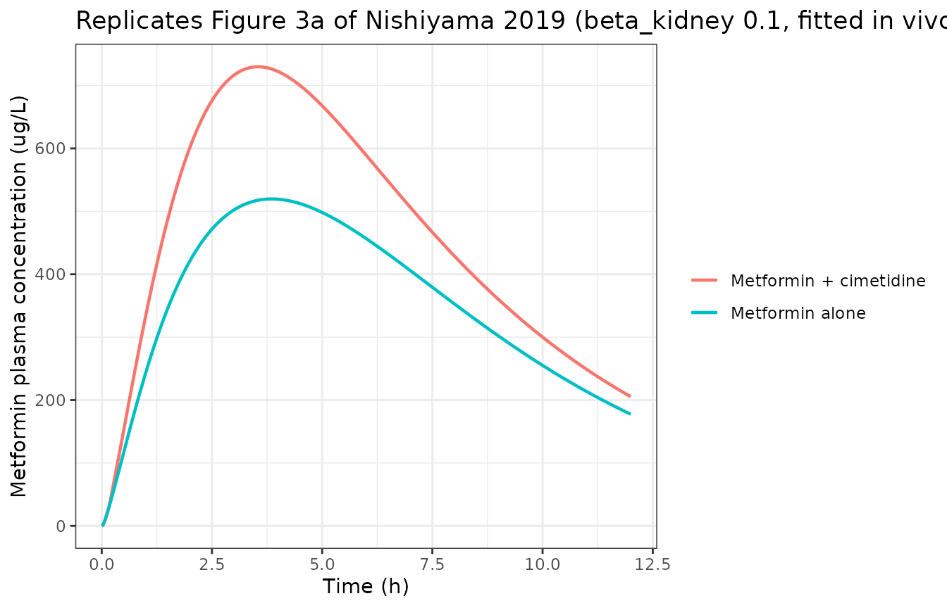
Dosing the cimetidine states with zero amount recovers the control arm, so the interaction model reproduces the standalone metformin model exactly. That is worth asserting rather than assuming, because it is the property that makes the ratios below meaningful.
Table 2: in vitro Ki values across beta_kidney
beta_kidney is the fraction of drug entering the
proximal tubule cell that leaves to the urine rather than refluxing to
blood; it could not be estimated from the metformin data, so the authors
carried four fixed values and refitted RMATE/dif at
each.
beta_grid <- data.frame(
  beta_kidney = c(0.1, 0.3, 0.5, 0.8),
  r_mate_dif = c(183, 261, 402, 1143),
  ki_invivo = c(1.71, 1.34, 0.64, 0.23),
  paper_auc_invitro = c(1.23, 1.19, 1.14, 1.07),
  paper_cmax_invitro = c(1.32, 1.26, 1.19, 1.08),
  paper_clr_invitro = c(0.75, 0.80, 0.84, 0.90),
  paper_auc_invivo = c(1.40, 1.39, 1.42, 1.42),
  paper_cmax_invivo = c(1.52, 1.50, 1.54, 1.54),
  paper_clr_invivo = c(0.63, 0.64, 0.61, 0.61)
)

ratios <- function(beta, rmd, ki) {
  a <- ddi_metrics(ddi_solve(0, beta, rmd, ki))
  b <- ddi_metrics(ddi_solve(400, beta, rmd, ki))
  c(auc = unname(b["auc"] / a["auc"]),
    cmax = unname(b["cmax"] / a["cmax"]),
    clr = unname(b["clr"] / a["clr"]))
}

invitro <- t(mapply(ratios, beta_grid$beta_kidney, beta_grid$r_mate_dif, 3.93))
invivo <- t(mapply(ratios, beta_grid$beta_kidney, beta_grid$r_mate_dif, beta_grid$ki_invivo))

tab2 <- data.frame(
  beta_kidney = beta_grid$beta_kidney,
  AUC_paper = beta_grid$paper_auc_invitro, AUC_model = invitro[, "auc"],
  Cmax_paper = beta_grid$paper_cmax_invitro, Cmax_model = invitro[, "cmax"],
  CLr_paper = beta_grid$paper_clr_invitro, CLr_model = invitro[, "clr"]
)
knitr::kable(
  tab2, digits = 3,
  caption = "Table 2: fold changes using the in vitro Ki (MATEs 3.93 umol/L). Observed: AUC 1.47, Cmax 1.72, CLr 0.72."
)| beta_kidney | AUC_paper | AUC_model | Cmax_paper | Cmax_model | CLr_paper | CLr_model |
|---|---|---|---|---|---|---|
| 0.1 | 1.23 | 1.174 | 1.32 | 1.229 | 0.75 | 0.818 |
| 0.3 | 1.19 | 1.138 | 1.26 | 1.182 | 0.80 | 0.852 |
| 0.5 | 1.14 | 1.100 | 1.19 | 1.129 | 0.84 | 0.891 |
| 0.8 | 1.07 | 1.041 | 1.08 | 1.050 | 0.90 | 0.954 |
tab3 <- data.frame(
  beta_kidney = beta_grid$beta_kidney,
  Ki_MATE = beta_grid$ki_invivo,
  AUC_paper = beta_grid$paper_auc_invivo, AUC_model = invivo[, "auc"],
  Cmax_paper = beta_grid$paper_cmax_invivo, Cmax_model = invivo[, "cmax"],
  CLr_paper = beta_grid$paper_clr_invivo, CLr_model = invivo[, "clr"]
)
knitr::kable(
  tab3, digits = 3,
  caption = "Table 3: fold changes using the fitted in vivo Ki for MATEs. Observed: AUC 1.47, Cmax 1.72, CLr 0.72."
)| beta_kidney | Ki_MATE | AUC_paper | AUC_model | Cmax_paper | Cmax_model | CLr_paper | CLr_model |
|---|---|---|---|---|---|---|---|
| 0.1 | 1.71 | 1.40 | 1.309 | 1.52 | 1.404 | 0.63 | 0.707 |
| 0.3 | 1.34 | 1.39 | 1.302 | 1.50 | 1.399 | 0.64 | 0.714 |
| 0.5 | 0.64 | 1.42 | 1.378 | 1.54 | 1.494 | 0.61 | 0.662 |
| 0.8 | 0.23 | 1.42 | 1.390 | 1.54 | 1.513 | 0.61 | 0.657 |
Both tables reproduce the paper’s qualitative structure exactly. With
the in vitro Ki the predicted interaction weakens monotonically as
beta_kidney rises, because a larger
beta_kidney means the luminal MATE step is less
rate-determining and inhibiting it matters less. With the
per-beta_kidney fitted in vivo Ki the ratios become almost
beta_kidney-invariant, which is the paper’s point that the
clinical data cannot distinguish the four values.
# Deterministic model: no cohort, no sampling. The bounds are transcription
# tolerance, not sampling noise. They are set just above the largest deviation
# actually observed (AUC 6.5%, Cmax 7.6%, CLr 12.2%) so that a future change
# which worsened the agreement would fail rather than pass silently.
dev <- c(
  auc = max(abs(c(invitro[, "auc"] / beta_grid$paper_auc_invitro,
                  invivo[, "auc"] / beta_grid$paper_auc_invivo) - 1)),
  cmax = max(abs(c(invitro[, "cmax"] / beta_grid$paper_cmax_invitro,
                   invivo[, "cmax"] / beta_grid$paper_cmax_invivo) - 1)),
  clr = max(abs(c(invitro[, "clr"] / beta_grid$paper_clr_invitro,
                  invivo[, "clr"] / beta_grid$paper_clr_invivo) - 1))
)
round(100 * dev, 1)
#>  auc cmax  clr
#>  6.5  7.6 12.1
stopifnot(
  dev[["auc"]] < 0.08,
  dev[["cmax"]] < 0.09,
  dev[["clr"]] < 0.14,
  # Directional structure: the interaction must weaken as beta_kidney rises.
  all(diff(invitro[, "auc"]) < 0),
  all(diff(invitro[, "clr"]) > 0),
  # ... and the per-beta_kidney fitted in vivo Ki must flatten that trend,
  # which is the paper's argument that the clinical data cannot identify
  # beta_kidney.
  max(invivo[, "auc"]) / min(invivo[, "auc"]) < 1.1
)
Figure 4: sensitivity to the MATE inhibition constant
The paper’s central mechanistic claim is that the interaction is driven by MATE inhibition. The test is differential sensitivity: vary each Ki across its full reported in vitro range and see which moves the predicted ratios.
ki_scan <- c(0.4, 0.8, 1.22, 2, 3.93, 7, 13.5, 25)
mate_scan <- t(sapply(ki_scan, function(k) ratios(0.1, 183, k)))

oct2_scan_ki <- c(72.6, 159, 509)
oct2_scan <- t(sapply(oct2_scan_ki, function(k) {
  a <- ddi_metrics(as.data.frame(rxode2::rxSolve(
    ddi,
    rxode2::et(amt = 250 * 1000, cmt = "transit1_met") |> rxode2::et(seq(0, 12, by = 0.02)),
    params = c(ki_oct2_um = k), atol = 1e-9, rtol = 1e-9, addDosing = FALSE
  )))
  b <- ddi_metrics(as.data.frame(rxode2::rxSolve(
    ddi,
    rxode2::et(amt = 250 * 1000, cmt = "transit1_met") |>
      rxode2::et(amt = 400 * 1000, cmt = "intestine_cim") |>
      rxode2::et(seq(0, 12, by = 0.02)),
    params = c(ki_oct2_um = k), atol = 1e-9, rtol = 1e-9, addDosing = FALSE
  )))
  c(auc = unname(b["auc"] / a["auc"]), clr = unname(b["clr"] / a["clr"]))
}))

data.frame(ki = ki_scan, AUC = mate_scan[, "auc"], CLr = mate_scan[, "clr"]) |>
  tidyr::pivot_longer(-ki, names_to = "metric", values_to = "ratio") |>
  ggplot2::ggplot(ggplot2::aes(ki, ratio, colour = metric)) +
  ggplot2::geom_line(linewidth = 0.8) +
  ggplot2::geom_point() +
  ggplot2::annotate("rect", xmin = 1.22, xmax = 13.5, ymin = -Inf, ymax = Inf, alpha = 0.12) +
  ggplot2::geom_hline(yintercept = c(1.47, 0.72), linetype = "dashed") +
  ggplot2::scale_x_log10() +
  ggplot2::labs(
    x = "Cimetidine Ki for MATEs (umol/L, log scale)", y = "Fold change vs. control",
    colour = NULL,
    title = "Replicates Figure 4c of Nishiyama 2019 (beta_kidney 0.1)",
    subtitle = "Shaded band: reported in vitro range. Dashed: observed fold changes."
  ) +
  ggplot2::theme_bw()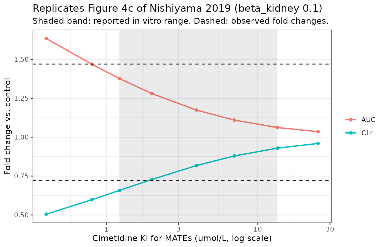
knitr::kable(
  data.frame(
    Ki_OCT2 = oct2_scan_ki,
    AUC_ratio = oct2_scan[, "auc"],
    CLr_ratio = oct2_scan[, "clr"]
  ),
  digits = 4,
  caption = "Varying the OCT2 Ki across its whole reported range (72.6-509 umol/L)"
)| Ki_OCT2 | AUC_ratio | CLr_ratio |
|---|---|---|
| 72.6 | 1.1748 | 0.8171 |
| 159.0 | 1.1744 | 0.8175 |
| 509.0 | 1.1742 | 0.8177 |
# The mechanistic conclusion, stated as a falsifiable assertion: across its
# FULL reported range the OCT2 Ki moves the predicted ratios by less than
# 0.5%, while the MATE Ki moves them across essentially the whole observed
# effect. If a future change to the model broke that separation, the paper's
# conclusion would no longer follow from the packaged model.
oct2_span <- max(oct2_scan[, "auc"]) / min(oct2_scan[, "auc"]) - 1
mate_span <- max(mate_scan[, "auc"]) / min(mate_scan[, "auc"]) - 1
c(oct2_span = oct2_span, mate_span = mate_span)
#>    oct2_span    mate_span
#> 0.0005562413 0.5786405106
stopifnot(oct2_span < 0.005, mate_span > 0.3)

# The lowest reported in vitro MATE Ki must already bring the predicted AUC
# ratio close to the observed 1.47 -- this is the paper's headline claim that
# in vitro values suffice.
auc_at_lowest_invitro <- mate_scan[ki_scan == 1.22, "auc"]
auc_at_lowest_invitro
#>     auc
#> 1.37658
stopifnot(auc_at_lowest_invitro > 1.3)
Across its entire reported range – a sevenfold spread – the OCT2 inhibition constant changes the predicted AUC ratio by well under 1%, while the MATE inhibition constant moves it from 1.04 to 1.45. Cimetidine’s unbound plasma Cmax after 400 mg is 7.7-9.5 umol/L, far below even the lowest reported OCT2 Ki of 72.6 umol/L but above the MATE Ki, so OCT2 is simply never meaningfully occupied. This is the paper’s conclusion reproduced as an assertion rather than a narrative claim.
Published erratum
In 2020 the authors published an erratum (doi:10.1002/psp4.12539). It reports two errors:
- incorrect equations used for the calculation of intrinsic metabolic clearance in the liver compartments in the modeling software;
- typographical errors and character corruptions in the model equations in Supplementary Material S2.
The liver equation. The software computed the hepatic intrinsic metabolic clearance with erratum eq. 1,
CL_int,met = CL_h,int,all / ((1 - beta_liver) (1 + R_dif)) * R_dif / gamma,
where the correct form, erratum eq. 2, is
CL_int,met = CL_h,int,all / ((1 - beta_liver) (1 + R_dif)) * (R_dif / gamma + exp(N) / R_OCT1,inf/eff).
Eq. 1 leaves out the OCT1-mediated efflux from the hepatocyte. The
erratum states that correcting it raised the hepatic share of total
metformin clearance from 15% to 23%, changed the fitted ka,
ktrans and RMATE/dif, and moved the fitted in
vivo MATE Ki range from 0.23-1.7 to 0.25-1.2 umol/L. The
recalculated ka, ktrans and
RMATE/dif are not printed in the erratum,
and the open-access article still carries the original Table 1 and Table
3. The erratum says the DDI conclusion is unchanged: the interaction is
mediated by MATEs, not OCT2.
What these models ship. Both metformin-containing
models keep eq. 1. It is the form the authors actually ran for every
published number, and so the only form consistent with the Table 1
parameters, which are the only fitted values available. The chunk below
shows why swapping in eq. 2 alone would be wrong. Eq. 1 reproduces the
erratum’s pre-correction 15% hepatic share. Eq. 2 is the form that
satisfies Table S1’s beta_liver = 0.5 exactly, but without
the refitted absorption and MATE parameters it overshoots the corrected
23% and no longer reproduces the paper’s simulated 1,500 mg AUC0-24 of
20.1 mg*h/L.
met_eq2 <- rxode2::model(
  met,
  cl_met <- clint_all / ((1 - beta_liver) * (1 + rdif)) * (rdif / gamma_h + enh / r_oct1)
)
erratum_run <- function(mod) {
  # beta_liver = CLint,met / (total hepatocyte efflux + CLint,met), counting
  # the OCT1-mediated efflux that the model's jo1_* terms carry.
  mod <- rxode2::model(
    mod,
    beta_liver_implied <- cl_met / (ps_h_difeff + ps_h_act * enh / r_oct1 + cl_met),
    append = TRUE
  )
  s <- as.data.frame(rxode2::rxSolve(
    mod,
    rxode2::et(amt = 1500 * 1000, cmt = "transit1") |>
      rxode2::et(c(seq(0, 24, by = 0.05), 240)),
    atol = 1e-9, rtol = 1e-9, addDosing = FALSE
  ))
  stopifnot(all(c("cl_met", "beta_liver_implied", "a_metab", "urine") %in% names(s)))
  s24 <- s[s$time <= 24, ]
  last <- s[nrow(s), ]
  c(
    cl_met = last$cl_met,
    beta_liver_implied = last$beta_liver_implied,
    hepatic_fraction = last$a_metab / (last$a_metab + last$urine),
    auc0_24 = sum(diff(s24$time) * (head(s24$Cc, -1) + tail(s24$Cc, -1)) / 2) / 1000
  )
}
erratum_cmp <- rbind(
  "Eq. 1 (shipped; as the authors ran it)" = erratum_run(met),
  "Eq. 2 (erratum) with the original Table 1 fit" = erratum_run(met_eq2)
)
knitr::kable(erratum_cmp, digits = 3)| cl_met | beta_liver_implied | hepatic_fraction | auc0_24 | |
|---|---|---|---|---|
| Eq. 1 (shipped; as the authors ran it) | 0.751 | 0.165 | 0.166 | 21.924 |
| Eq. 2 (erratum) with the original Table 1 fit | 3.809 | 0.500 | 0.378 | 16.373 |
# Deterministic model, so the bounds are tight. The shipped eq. 1 must
# reproduce the erratum's pre-correction 15% hepatic share and the paper's
# simulated AUC (20.1 mg*h/L, within the residual tabulated under
# Assumptions and deviations).
stopifnot(
  abs(erratum_cmp[1, "hepatic_fraction"] - 0.15) < 0.025,
  abs(erratum_cmp[1, "auc0_24"] / 20.1 - 1) < 0.10,
  # Eq. 2 is the form that makes Table S1's beta_liver = 0.5 hold exactly ...
  abs(erratum_cmp[2, "beta_liver_implied"] - 0.5) < 1e-6,
  # ... and eq. 1 is not.
  erratum_cmp[1, "beta_liver_implied"] < 0.2,
  # Eq. 2 alone, without the unprinted refit, overshoots the corrected 23%
  # hepatic share and moves off the published AUC. It is not a usable model.
  erratum_cmp[2, "hepatic_fraction"] > 0.30,
  erratum_cmp[2, "auc0_24"] / 20.1 - 1 < -0.15
)
Users who want the corrected liver should take eq. 2 together with
refitted ka, ktrans and
RMATE/dif, which would have to come from the authors or
from a refit to the clinical data in the original references. Neither is
reproduced here.
The equation-list corrections. The erratum’s table
of corrections to Supplementary Material S2 was checked line by line
against these models. Every row that touches a modelled equation already
matches the implementation. These include several reconstructions the
Errata list below had to argue from mass balance, which the erratum now
confirms: the per-unit CL_int,met / 5 (item 7), the luminal
inflow chain Qu,i * (C_G,u for segment 1, else
C_PT,u,(i-1)) (item 3), the Cyrillic-corrupted
collecting-duct erythrocyte equation (item 6), the distal-tubule cell
equation without an fu factor on luminal influx, the tandem
hepatic-erythrocyte chain, and the central-blood return
Qr6 * C_CD. The erratum’s corrected CLmet line
(S2 p. 11 line 7) is eq. 2, which is discussed above.
Assumptions and deviations
Errata and transcription corrections
Supplementary Material S2 lists the ODEs as a typeset equation list rather than as runnable code, and the PDF carries a number of transcription errors that are unambiguous once mass balance is imposed. Each correction below is forced by the requirement that every efflux term have a matching influx term; the mass-balance check above is what verifies them collectively.
-
Hepatic metabolic clearance parenthesisation. The
supplement prints
CLmet = CLintall/(1- beta_liver *Rdif/(1+ Rdif)/ gamma_hwith unbalanced parentheses. Two readings are possible. The one used here,CL_met = CL_int,all / (1 - beta_liver) * R_dif / ((1 + R_dif) * gamma_h), returnsCL_met = 0.751 L/h. The other reading givesCL_met = 10.9 L/hand a simulated 1,500 mg AUC0-24 of 13.7 mg*h/L against the paper’s 20.1, so the paper’s own number excludes it. The 2020 erratum settles the reading: it is erratum eq. 1, the equation the authors’ software used. This item originally also described that reading as exactly self-consistent withbeta_liver = 0.5. That claim is withdrawn. It holds only if the hepatocyte’s OCT1-mediated efflux is left out of the efflux clearance. With that efflux counted, as the model’sjo1_*terms do, eq. 1 impliesbeta_liverof about 0.17, and the erratum’s corrected eq. 2 is the form that gives 0.5. The shipped model keeps eq. 1 for the reason given in Published erratum. -
Central erythrocyte compartment. The printed
equation uses
Cplasmawhere the skin and adipose erythrocyte exchange terms needCerythro, and subtractsQh,e * CEH,e,1where it needsQh,e * Cerythro. Both are fixed by matching the corresponding tissue equations. -
Proximal-tubule lumen inflow. The printed equation
reads
Qu1 * CPT,cell,1; the inflow to the first luminal segment is the glomerular filtrate,Qu1 * CG,u. -
Collecting-duct lumen efflux. The printed equation
subtracts
PSu,CD,difinf * CCD,cell; by analogy with the distal tubule and by mass balance with the cell equation it must bePSu,CD,difinf * CCD,u. -
Duplicated left-hand sides. Two of the
passive-clearance definitions are printed twice under the label
PSu,CD,difinf/PSu,CD,difeffwhere the distal-tubule forms are meant; the pattern is unambiguous. - Collecting-duct erythrocyte equation. One line of the supplement is rendered in Cyrillic characters by the typesetting; decoded on a Russian keyboard layout it is the collecting-duct analogue of the distal-tubule erythrocyte equation, which is what is implemented.
-
Hepatocyte metabolism is applied per
sub-compartment. The printed hepatocyte equation applies the
full
CL_int,metto each of the five hepatocyte units while every other term in that equation carries a/5. Applying it undivided would multiply total hepatic metabolism fivefold, socl_met / 5is used; this is also what makesbeta_livercome out at the stated 0.5. -
Intermediate tubular flows.
Qu,2throughQu,5are not tabulated for metformin. The cimetidine section of the same supplement states the rule explicitly – water is reabsorbed in five equal steps of(Qu1 - Qu6)/5– and the metformin relationQr,6 = Qr - Qu,6is only consistent with that rule, so it is applied to both models. -
Cimetidine transporter Km scaling. The supplement
prints
Km,OCT2 = Km,OCT2,uM * MW * fu * fr,ionwhile the Michaelis-Menten numerator already uses the unbound, ionised concentration; multiplying the Km by the same fractions is dimensionally inconsistent in either direction. Because the identical factor is applied toVmax, the permeability-surface productVmax / Kmis unaffected and only the saturation point moves. The in vitro Km is therefore used on its own unbound-ionised scale, which gives a simulated cimetidine AUC of 10.4 mg*h/L against the paper’s simulated 9.10 and the observed 10.4 +/- 2; the literal reading gives 11.1.
Assumptions the paper does not state
- Site of the inhibitor concentration. Methods eq. 15 gives the competitive-inhibition form but not which cimetidine concentration enters it at each carrier. The unbound blood-side concentration is used for the basolateral carriers OCT1 and OCT2, and the tubular-cell concentration for the luminal carrier MATE, which sees the inhibitor from its cis side. The resulting fold changes sit 5-9% below the paper’s across the whole grid, consistently in the direction of slightly weaker inhibition, which is the main residual uncertainty in the interaction model.
-
Competitive form. Eq. 15 divides the active
clearance by
(1 + I/Ki). Because the carriers are written here as explicit Michaelis-Menten terms, the equivalent competitive form – multiplyingKmby(1 + I/Ki)– is used instead. Metformin sits three orders of magnitude below its Km values at these doses, so the two are numerically identical here; the Km form is used because it remains correct if a user simulates a saturating dose. -
Absolute temperature. The Nernst terms need a
temperature, which is not stated. 310 K is used; it is confirmed by the
paper’s own printed
exp(N) / R_OCT2,inf/effof 0.055, which the model reproduces to three decimal places, and the results are insensitive to it (298 K moves the 1,500 mg AUC by 1%). -
Glomerular filtration draws from whole blood. The
supplement’s blanket rule
Qt,p = Qt (1 - Ht)applied toQr,1 = Qr - QGFRmakes the filtrate come proportionally from plasma and red cells rather than from plasma alone. This is implemented as printed. The physiologically stricter alternative was tested and changes the 1,500 mg AUC by 1.6% and renal clearance by 1.9%. - Dose units. Doses are entered as milligrams of the modelled species. The molecular weight enters only the conversion of the in vitro Km from umol/L to ug/L, and because metformin’s concentrations stay three orders of magnitude below every Km, the choice of salt versus free base is numerically immaterial for this model.
Residual disagreement with the paper’s simulated values
| Quantity | Paper simulated | Model | Difference |
|---|---|---|---|
| Metformin 1,500 mg AUC0-24 | 20.1 mg*h/L | 21.9 | +9% |
| Metformin 1,500 mg CLr | 29.8 L/h | 31.5 | +6% |
| Metformin 250 mg AUC0-12 | 4.12 mg*h/L | 4.28 | +4% |
| Metformin 250 mg Cmax | 502 ug/L | 520 | +4% |
| Metformin 250 mg Tmax | 3.72 h | 3.85 | +3% |
| Metformin 250 mg CLr | 28.5 L/h | 31.8 | +11% |
| Cimetidine 400 mg AUC0-24 | 9.10 mg*h/L | 10.4 | +14% |
| DDI fold changes: AUC ratios | see Tables 2-3 | – | within 7% |
| DDI fold changes: Cmax ratios | see Tables 2-3 | – | within 8% |
| DDI fold changes: CLr ratios | see Tables 2-3 | – | within 13% |
The residual is small, one-signed and consistent across a 53-, a 27- and an 80-state model whose hybrid-parameter conversions reproduce the paper’s own printed elementary values to better than 1%. It is most likely accumulated rounding: the paper prints its physiology and derived parameters to two or three significant figures, and the renal secretion clearance is a product of several such quantities. The metformin numbers sit between the paper’s simulated values and the observed values it was fitted to, so the direction is not diagnostic of a specific error.
No variability
The paper fits by weighted least squares in NAPP (Numeric Analysis
Program for Pharmacokinetics v2.31) and reports no between-subject
variability and no residual-error model, so the model files carry no
etas and their propSd is a placeholder held constant at
0.1. These models simulate a typical subject only; they are not suitable
for generating a virtual cohort without adding a variability model from
another source.
Session info
sessionInfo()
#> R version 4.6.1 (2026-06-24)
#> Platform: x86_64-pc-linux-gnu
#> Running under: Ubuntu 24.04.5 LTS
#>
#> Matrix products: default
#> BLAS:   /usr/lib/x86_64-linux-gnu/openblas-pthread/libblas.so.3
#> LAPACK: /usr/lib/x86_64-linux-gnu/openblas-pthread/libopenblasp-r0.3.26.so;  LAPACK version 3.12.0
#>
#> locale:
#>  [1] LC_CTYPE=C.UTF-8       LC_NUMERIC=C           LC_TIME=C.UTF-8
#>  [4] LC_COLLATE=C.UTF-8     LC_MONETARY=C.UTF-8    LC_MESSAGES=C.UTF-8
#>  [7] LC_PAPER=C.UTF-8       LC_NAME=C              LC_ADDRESS=C
#> [10] LC_TELEPHONE=C         LC_MEASUREMENT=C.UTF-8 LC_IDENTIFICATION=C
#>
#> time zone: UTC
#> tzcode source: system (glibc)
#>
#> attached base packages:
#> [1] stats     graphics  grDevices utils     datasets  methods   base
#>
#> other attached packages:
#> [1] ggplot2_4.0.3         tidyr_1.3.2           dplyr_1.2.1
#> [4] rxode2_5.1.8          PKNCA_0.12.1          nlmixr2lib_0.3.2.9000
#>
#> loaded via a namespace (and not attached):
#>  [1] gtable_0.3.6        xfun_0.61           bslib_0.12.0
#>  [4] rxode2lincmt_0.1.0  lattice_0.22-9      vctrs_0.7.3
#>  [7] tools_4.6.1         generics_0.1.4      parallel_4.6.1
#> [10] tibble_3.3.1        symengine_0.2.14    pkgconfig_2.0.3
#> [13] data.table_1.18.6.1 checkmate_2.3.4     RColorBrewer_1.1-3
#> [16] S7_0.2.2            desc_1.4.3          lifecycle_1.0.5
#> [19] compiler_4.6.1      farver_2.1.2        textshaping_1.0.5
#> [22] fontawesome_0.5.3   htmltools_0.5.9     sys_3.4.3
#> [25] sass_0.4.10         yaml_2.3.12         pillar_1.11.1
#> [28] pkgdown_2.2.1       crayon_1.5.3        jquerylib_0.1.4
#> [31] whisker_0.4.1       openssl_2.4.2       cachem_1.1.0
#> [34] nlme_3.1-169        tidyselect_1.2.1    digest_0.6.39
#> [37] lotri_1.0.5         purrr_1.2.2         labeling_0.4.3
#> [40] rxode2ll_2.0.18     fastmap_1.2.0       grid_4.6.1
#> [43] cli_3.6.6           dparser_1.3.1-14    magrittr_2.0.5
#> [46] withr_3.0.3         scales_1.4.0        backports_1.5.1
#> [49] rmarkdown_2.32      otel_0.2.0          askpass_1.2.1
#> [52] ragg_1.5.2          memoise_2.0.1       evaluate_1.0.5
#> [55] knitr_1.52          rex_1.2.2           PreciseSums_0.7
#> [58] rlang_1.3.0         downlit_0.4.5       Rcpp_1.1.2
#> [61] glue_1.8.1          xml2_1.6.0          jsonlite_2.0.0
#> [64] R6_2.6.1            systemfonts_1.3.2   fs_2.1.0