Magnesium sulfate exposure-response for eclampsia (Du 2019)

Source and model

• Citation: Du L, Wenning LA, Carvalho B, Duley L, Brookfield KF, Witjes H, de Greef R, Lumbiganon P, Titapant V, Kongwattanakul K, Long Q, Sangkomkamhang US, Gulmezoglu AMG, Oladapo OT. Alternative magnesium sulfate dosing regimens for women with preeclampsia: a population pharmacokinetic exposure-response modeling and simulation study. J Clin Pharmacol. 2019;59(11):1519-1526. doi:10.1002/jcph.1448. PMCID PMC6790709. The clearance function that generates the exposure metric is restated in this paper (Methods, Pharmacokinetic Exposure and Supplemental Table S1) from the companion population PK analysis: Du L, Wenning L, Migoya E, et al. Population pharmacokinetic modeling to evaluate standard magnesium sulfate treatments and alternative dosing regimens for women with preeclampsia. J Clin Pharmacol. 2019;59(3):374-385. doi:10.1002/jcph.1328.
• Article (open access): https://doi.org/10.1002/jcph.1448
• PubMed Central: https://www.ncbi.nlm.nih.gov/pmc/articles/PMC6790709/
• Supporting Information (Figures S1-S6, Tables S1-S5): distributed with the article and retrieved from the Europe PMC supplementary-files endpoint for PMC6790709.

Magnesium sulfate is the anticonvulsant of choice for preventing and treating eclampsia, but the two standard regimens – the intravenous Zuspan regimen and the predominantly intramuscular Pritchard regimen – require either a controlled infusion pump for 24 hours or six large-volume intramuscular injections. Since 2013 the World Health Organization has been looking for simpler alternatives that would be deliverable in resource-limited settings. Du 2019 supports that initiative by quantifying how the probability of eclampsia falls with magnesium exposure, then simulating that probability for the standard regimens and for eighteen alternatives.

This package carries one model from this paper: the exposure-response logistic regression. The paper describes itself as the second part of a two-part project; the first part – the population pharmacokinetic model that supplies the clearance function – was published separately as doi:10.1002/jcph.1328 and is restated here only in Supplemental Table S1. See Assumptions and deviations below for what that means for the Table 1 Cmax column.

Model file	What it is	Source
Du_2019_magnesiumSulfate_eclampsia	Landmark logistic exposure-response for eclampsia occurrence, with the closed-form exposure metric built in	Methods (Pharmacokinetic Exposure, E-R Model Development), Results (Exposure-Response Model Results), Table S1

Population

Exposure-response analysis population (Du 2019 Tables S2 and S3).

Field	Value
Species	human
Women	10280
Studies	2
Observations	10280 binary eclampsia records (one per woman; landmark analysis, no repeated measures). 127 women developed eclampsia: 37 on magnesium sulfate (36 Magpie, 1 Thai) and 90 on placebo (all Magpie).
Age	Magpie median 26 years (P5-P95 17-39); Thailand median 28 years (P5-P95 17-40)
Body weight	Thailand median 73 kg (P5-P95 54-103); not collected in Magpie, imputed at the Stanford median of 85 kg
Disease	preeclampsia; Magpie women had not given birth or were within 24 h postpartum (median gestational age 37 weeks, P5-P95 27-41), Thai women had median gestational age 38 weeks (P5-P95 31-40)
Regimens	Magpie: 4 g IV loading then either 1 g/h IV for 24 h, or 10 g IM loading plus 5 g IM every 4 h for 24 h, or matching placebo. Thailand: 4 g IV loading then 1 g/h IV infusion. Simulated regimens span 6-54 g total per 24 h (Table S4).
Regions	Magpie Trial: multicentre randomised trial across 33 countries (1998-2001). Thai study: Srinagarind Hospital (Khon Kaen University) and Siriraj Hospital (Mahidol University), Thailand (2010-2013).

Three studies feed the two-part project, and they do not overlap:

• Stanford (2012-2014, n = 92). Rich serial magnesium sampling under intravenous treatment; the only study with concentration data, and the only one used to fit the population PK model. No eclampsia outcomes.
• Magpie Trial (1998-2001, n = 9891 in this analysis). A placebo-controlled randomised trial across 33 countries. Eclampsia outcomes only – no magnesium concentrations, and neither body weight nor serum creatinine was collected, so Du 2019 assigned every Magpie woman the Stanford medians of 85 kg and 0.8 mg/dL.
• Thai study (2010-2013, n = 389). Sparse post-dose magnesium samples and eclampsia outcomes. Weight available in 383 women, serum creatinine in 168; missing values imputed at the Thai medians of 73 kg and 0.6 mg/dL.

The consequence is worth stating plainly, because it bounds what this model can be used for: no individual serum magnesium concentration in the exposure-response analysis set informs its own AUC. For the Magpie women the AUC is a deterministic function of total dose and route alone. Du 2019’s own sensitivity check – imputing 80 kg and 0.7 mg/dL instead of 85 kg and 0.8 mg/dL moved the AUC by about 5% – is reported in the Results as reassurance on that point.

Source trace

Source location for every value in the model file.

Quantity	Value	Source location
CL typical value	3.72 L/h	Methods (Pharmacokinetic Exposure) equation; Table S1 row ‘CL (L/h)’, RSE 3.5%
Serum creatinine exponent on CL	-0.731	Table S1 row ‘Serum creatinine exponent for CL, theta’, RSE 14.2%; Methods equation writes the equivalent (0.8 mg/dL / Cr)^0.731
Body weight exponent on CL	0.75 (fixed)	Table S1 row ‘WT exponent for CL and Q’; Methods equation (WT/85 kg)^0.75
CL reference creatinine	0.8 mg/dL	Methods equation; Stanford cohort median
CL reference weight	85 kg	Methods equation; Stanford cohort median
AUC definition	DOSE_IV/CL and F*DOSE_IM/CL	Methods (Pharmacokinetic Exposure) equations
Intramuscular bioavailability F	0.862	Methods (Pharmacokinetic Exposure): ‘estimated as 0.862 based on the published literature’, citing Salinger 2013 (reference 7)
Elemental Mg content of the salt	~10% (0.098612 exact)	Table 1 footnote: ‘Dosage form in simulated dosing regimen was MgSO4-7H2O, which contains ~10% of magnesium’
Logit intercept, age <= 22 y	-6.29	Results (Exposure-Response Model Results), first printed branch
Logit intercept, age > 22 y	-4.72	Results (Exposure-Response Model Results), second printed branch
AUC coefficient	-0.00164	Results, both printed branches
Age coefficient, age <= 22 y	0.154	Results, first printed branch
Age coefficient, age > 22 y	0.010	Results, second printed branch
Age knot	22 years	Results: ‘a piece-wise linear age effect with a knot point at 22 years’
Placeholder residual SD	0.001 (fixed)	NOT from source; see Assumptions and deviations

Model structure

The model has no ODE and no time dimension. Everything below is evaluated once per woman.

Exposure. Du 2019 does not integrate a solved concentration profile. It computes the total (zero to infinity) area under the change-from-baseline serum magnesium curve in closed form, which for a linear disposition is exactly dose over clearance:

$$CL_i = 3.72 \cdot \left(\frac{0.8\ \text{mg/dL}}{Cr_i}\right)^{0.731} \cdot \left(\frac{WT_i}{85\ \text{kg}}\right)^{0.75}, \qquad AUC_i = \frac{DOSE_{IV,i} + F \cdot DOSE_{IM,i}}{CL_i}$$

That is why no volume, intercompartmental clearance or absorption rate constant appears anywhere in the model file: the AUC simply does not depend on them. Doses enter as grams of the administered salt MgSO4-7H2O and are converted to milligrams of elemental magnesium inside model().

Response. A logistic regression with a piece-wise linear age effect, knot at 22 years. Du 2019 prints the final model as two branches:

Age <= 22 years: Logit(P) = -6.29 - 0.00164 * AUC + 0.154 * age
Age >  22 years: Logit(P) = -4.72 - 0.00164 * AUC + 0.010 * age

The two printed branches are not continuous at the knot. The Methods equation is written in the continuous form b0 + b1*AUC + b2*Age + delta*(Age - k)*I(Age > k), which is continuous by construction, but the published coefficients are not consistent with it: at age 22 and AUC 0 the lower branch gives a logit of -2.902 and the upper branch -4.500, a jump of 1.598 logit units, or roughly a five-fold drop in predicted risk on crossing a birthday. Solving for a knot that would make the printed branches continuous gives 10.9 years, not 22.

The branches are nevertheless encoded exactly as printed, because they are what generated the paper’s own Table 1 – the check below reproduces all 18 regimen rows of both predicted-rate columns. No erratum exists.

The published branches disagree at the knot.

Branch	Logit	Probability at AUC = 0
age <= 22 (evaluated at 22)	-2.902	0.0521
age > 22 (evaluated at 22)	-4.500	0.0110

Reproducing Table 1

Du 2019 simulated 27 “types” of woman – every combination of age (20, 30, 40 years), body weight (60, 85, 110 kg) and serum creatinine (0.5, 0.8, 1.2 mg/dL) – and reports, for each regimen, the mean predicted eclampsia rate across all 27 and across the 18 aged over 22. Table S4 gives the regimens; the total doses below are read from the Table 1 Total Dose column and split by route according to each regimen’s description.

# Regimen definitions. dose_iv / dose_im are TOTAL grams of MgSO4-7H2O over
# the course, per Du 2019 Table 1 (Total Dose column) and Table S4.
regimens <- tibble::tribble(
  ~regimen,                                        ~route, ~dose_iv, ~dose_im, ~pub_all, ~pub_gt22,
  "Placebo",                                       "None",        0,        0,      2.1,      1.2,
  "4 g in 20 min, 1 g/h x 24 h (Zuspan)",          "IV",         28,        0,     0.64,     0.37,
  "4 g in 20 min, 2 g/h x 24 h",                   "IV",         52,        0,     0.25,     0.15,
  "6 g in 20 min, 2 g/h x 24 h",                   "IV",         54,        0,     0.24,     0.14,
  "12 g in 120 min, 3 g/h x 12 h",                 "IV",         48,        0,     0.29,     0.17,
  "12 g in 120 min, 2 g/h x 8 h",                  "IV",         28,        0,     0.64,     0.37,
  "8 g in 60 min, 2 g/h x 10 h",                   "IV",         28,        0,     0.64,     0.37,
  "4 g in 20 min, 1 g/h x 12 h",                   "IV",         16,        0,      1.0,     0.61,
  "4 g in 20 min, 1 g/h x 8 h",                    "IV",         12,        0,      1.2,     0.73,
  "6 g in 20 min",                                 "IV",          6,        0,      1.6,     0.94,
  "4 g IV/10 g IM, 5 g Q4h x 5 (Pritchard)",       "IM",          4,       35,     0.50,     0.29,
  "4 g IV/10 g IM, 8 g Q6h x 3",                   "IM",          4,       34,     0.52,     0.30,
  "4 g IV/10 g IM, 10 g Q8h x 2",                  "IM",          4,       30,     0.59,     0.35,
  "4 g IV/10 g IM, 5 g Q4h x 2",                   "IM",          4,       20,     0.84,     0.49,
  "4 g IV/10 g IM",                                "IM",          4,       10,      1.2,     0.71,
  "10 g IM",                                       "IM",          0,       10,      1.4,     0.84,
  "10 g IM Q12h x 2",                              "IM",          0,       20,      1.0,     0.58,
  "10 g IM Q8h x 3",                               "IM",          0,       30,     0.70,     0.41,
  "4 g IV/6 g IM",                                 "IM",          4,        6,      1.4,     0.82
)

# Every split reproduces the Table 1 Total Dose column.
stopifnot(all(regimens$dose_iv + regimens$dose_im ==
                c(0, 28, 52, 54, 48, 28, 28, 16, 12, 6,
                  39, 38, 34, 24, 14, 10, 20, 30, 10)))

# The 27 "types" of woman, Du 2019 Model Simulations.
women <- expand.grid(
  AGE = c(20, 30, 40), WT = c(60, 85, 110), CREAT = c(0.5, 0.8, 1.2)
)
stopifnot(nrow(women) == 27L)

solve_regimen <- function(dose_iv, dose_im) {
  ev <- data.frame(
    id = seq_len(nrow(women)), time = 0, amt = 0, evid = 0L,
    AGE = women$AGE, WT = women$WT, CREAT = women$CREAT,
    DOSE_MGSO4_IV_G = dose_iv, DOSE_MGSO4_IM_G = dose_im
  )
  as.data.frame(rxode2::rxSolve(mod, events = ev, returnType = "data.frame"))
}

per_woman <-
  regimens |>
  dplyr::rowwise() |>
  dplyr::reframe(
    regimen = regimen, route = route,
    solve_regimen(dose_iv, dose_im) |>
      dplyr::select(AGE, WT, CREAT, auc_mg, prob_eclampsia)
  )
#> Warning: There were 19 warnings in `dplyr::reframe()`.
#> The first warning was:
#> ℹ In argument: `dplyr::select(...)`.
#> ℹ In row 1.
#> Caused by warning:
#> ! multi-subject simulation without without 'omega'
#> ℹ Run `dplyr::last_dplyr_warnings()` to see the 18 remaining warnings.

table1 <-
  per_woman |>
  dplyr::group_by(regimen, route) |>
  dplyr::summarise(
    sim_all  = 100 * mean(prob_eclampsia),
    sim_gt22 = 100 * mean(prob_eclampsia[AGE > 22]),
    .groups = "drop"
  ) |>
  dplyr::right_join(regimens, by = c("regimen", "route")) |>
  dplyr::mutate(
    total = dose_iv + dose_im,
    diff_all  = sim_all  - pub_all,
    diff_gt22 = sim_gt22 - pub_gt22
  ) |>
  dplyr::arrange(match(regimen, regimens$regimen))

Predicted mean eclampsia rate, this model versus Du 2019 Table 1.

Regimen	Total dose (g)	Simulated, all ages (%)	Du 2019, all ages (%)	Simulated, age > 22 y (%)	Du 2019, age > 22 y (%)
Placebo	0	2.127	2.10	1.251	1.20
4 g in 20 min, 1 g/h x 24 h (Zuspan)	28	0.646	0.64	0.376	0.37
4 g in 20 min, 2 g/h x 24 h	52	0.255	0.25	0.148	0.15
6 g in 20 min, 2 g/h x 24 h	54	0.237	0.24	0.137	0.14
12 g in 120 min, 3 g/h x 12 h	48	0.296	0.29	0.172	0.17
12 g in 120 min, 2 g/h x 8 h	28	0.646	0.64	0.376	0.37
8 g in 60 min, 2 g/h x 10 h	28	0.646	0.64	0.376	0.37
4 g in 20 min, 1 g/h x 12 h	16	1.060	1.00	0.618	0.61
4 g in 20 min, 1 g/h x 8 h	12	1.257	1.20	0.734	0.73
6 g in 20 min	6	1.630	1.60	0.955	0.94
4 g IV/10 g IM, 5 g Q4h x 5 (Pritchard)	39	0.505	0.50	0.293	0.29
4 g IV/10 g IM, 8 g Q6h x 3	38	0.522	0.52	0.304	0.30
4 g IV/10 g IM, 10 g Q8h x 2	34	0.599	0.59	0.348	0.35
4 g IV/10 g IM, 5 g Q4h x 2	24	0.851	0.84	0.496	0.49
4 g IV/10 g IM	14	1.224	1.20	0.715	0.71
10 g IM	10	1.454	1.40	0.851	0.84
10 g IM Q12h x 2	20	1.006	1.00	0.587	0.58
10 g IM Q8h x 3	30	0.704	0.70	0.410	0.41
4 g IV/6 g IM	10	1.420	1.40	0.831	0.82

# Deterministic typical-value arithmetic on a fixed 27-point covariate grid:
# no random draws anywhere, so tight absolute bounds are the right assertion.
stopifnot(
  # Every one of the 36 published cells is matched. The published values are
  # printed to 1 or 2 decimal places and Du 2019 appears to truncate rather
  # than round, which sets the floor on how tight this can be.
  max(abs(table1$diff_all))  < 0.07,
  max(abs(table1$diff_gt22)) < 0.07,
  # ... and the agreement is tight RELATIVE to the values too, which the
  # absolute bound alone would not show for the sub-0.3% regimens.
  max(abs(table1$diff_all  / table1$pub_all))  < 0.06,
  max(abs(table1$diff_gt22 / table1$pub_gt22)) < 0.06,
  # The efficacy criterion Du 2019 applies (mean rate at most 0.7%) partitions
  # the 19 rows identically whether it is applied to the simulated or to the
  # published column.
  identical(round(table1$sim_all, 2) <= 0.70, table1$pub_all <= 0.70),
  # The three intramuscular alternatives Du 2019 singles out in the Abstract
  # and Conclusions all clear the criterion.
  all(round(table1$sim_all[table1$regimen %in% c(
    "4 g IV/10 g IM, 8 g Q6h x 3",
    "4 g IV/10 g IM, 10 g Q8h x 2",
    "10 g IM Q8h x 3"
  )], 2) <= 0.70),
  # The paper's headline number for the intramuscular-only alternative.
  abs(round(table1$sim_all[table1$regimen == "10 g IM Q8h x 3"], 2) - 0.70) < 1e-8
)

# A mutation control: the gate above is not vacuous. Dropping the intramuscular
# bioavailability to 1 (i.e. mis-transcribing F) must break the IM rows.
mutated <- regimens |>
  dplyr::filter(route == "IM") |>
  dplyr::rowwise() |>
  dplyr::reframe(
    regimen = regimen, pub_all = pub_all,
    p = mean(solve_regimen(dose_iv, dose_im / 0.862)$prob_eclampsia)
  ) |>
  dplyr::mutate(diff = 100 * p - pub_all)
#> Warning: There were 9 warnings in `dplyr::reframe()`.
#> The first warning was:
#> ℹ In argument: `p = mean(solve_regimen(dose_iv,
#>   dose_im/0.862)$prob_eclampsia)`.
#> ℹ In row 1.
#> Caused by warning:
#> ! multi-subject simulation without without 'omega'
#> ℹ Run `dplyr::last_dplyr_warnings()` to see the 8 remaining warnings.
stopifnot(max(abs(mutated$diff)) > 0.07)

All 36 cells agree, and the mutation control confirms the gate discriminates: setting the intramuscular bioavailability to 1 moves the intramuscular rows by 0.10 percentage points, well outside the tolerance.

Reproducing the reported AUC estimates

Du 2019 reports the median estimated AUC in the Magpie Trial as 769 mgh/L for the intravenous maintenance arm and 906 mgh/L for the intramuscular arm. Every Magpie woman carries the imputed 85 kg and 0.8 mg/dL, so her clearance is exactly the typical 3.72 L/h and her AUC is a function of total dose alone – which makes this an independent check on the elemental-magnesium conversion and on the intramuscular bioavailability, neither of which the Table 1 gate could separate from the logistic coefficients.

magpie <- function(dose_iv, dose_im) {
  ev <- data.frame(
    id = 1L, time = 0, amt = 0, evid = 0L,
    AGE = 26, WT = 85, CREAT = 0.8,
    DOSE_MGSO4_IV_G = dose_iv, DOSE_MGSO4_IM_G = dose_im
  )
  as.data.frame(rxode2::rxSolve(mod, events = ev, returnType = "data.frame"))$auc_mg
}

auc_check <- tibble::tibble(
  Arm = c("Magpie IV maintenance (Zuspan, 28 g)",
          "Magpie IM maintenance (Pritchard, 4 g IV + 35 g IM)"),
  Simulated = c(magpie(28, 0), magpie(4, 35)),
  `Du 2019 median` = c(769, 906)
) |>
  dplyr::mutate(`Difference (%)` = 100 * (Simulated / `Du 2019 median` - 1))

knitr::kable(auc_check, digits = 1,
             caption = "Estimated AUC for the planned Magpie regimens.")

Estimated AUC for the planned Magpie regimens.

Arm	Simulated	Du 2019 median	Difference (%)
Magpie IV maintenance (Zuspan, 28 g)	742.2	769	-3.5
Magpie IM maintenance (Pritchard, 4 g IV + 35 g IM)	905.8	906	0.0

stopifnot(
  # The intramuscular arm lands on the published median to better than 0.1%.
  # Both F = 0.862 and the 0.098612 g/g elemental-magnesium fraction have to be
  # right for this to happen: perturbing either by 1% moves it by about 9 mg*h/L.
  abs(auc_check$Simulated[2] - 906) < 1,
  # The intravenous arm is 3.6% below the published median, because the planned
  # 28 g understates what the median Magpie woman actually received (Du 2019
  # used "the total MgSO4 dose administered up to the day of first eclampsia",
  # which varied with treatment duration). 769 mg*h/L implies 29.0 g.
  abs(auc_check$Simulated[1] - 769) < 30,
  auc_check$Simulated[1] < 769
)

# What total intravenous dose would give the published median exactly?
implied_g <- 769 * 3.72 / (1000 * 0.098612)
stopifnot(implied_g > 28, implied_g < 30)

The intramuscular arm matches to 0.20 mg*h/L; the intravenous arm implies a median administered dose of 29.0 g against the planned 28 g, consistent with Du 2019 using each woman’s actual cumulative dose.

Replicating Figure 1

Figure 1 overlays observed and model-predicted eclampsia rates against estimated AUC (left) and against age (right). The observed points and their confidence intervals are not tabulated anywhere in the article or supplement, so only the model curve is reproduced here, annotated with the AUC quantile boundaries the figure legend gives and with the two observed rates the text does print: 2.1% under placebo and 0.7% overall under magnesium sulfate (37 of 5290).

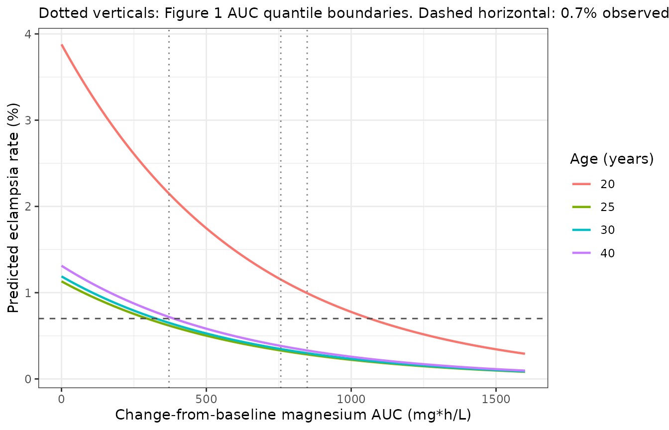
Replicates the left panel of Figure 1 of Du 2019: predicted eclampsia rate against change-from-baseline magnesium AUC, by age.

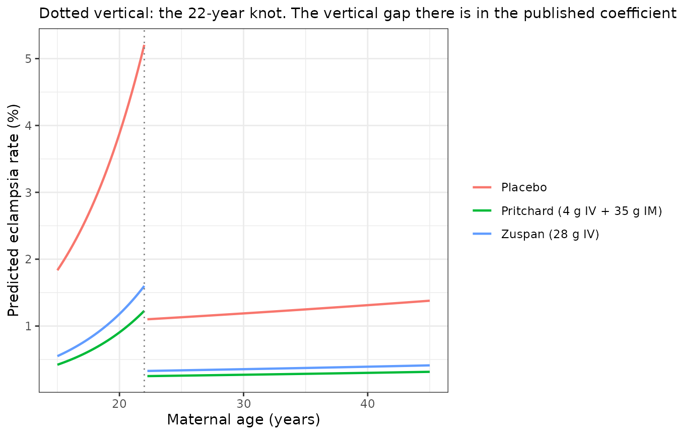
Replicates the right panel of Figure 1 of Du 2019: predicted eclampsia rate against age, at the AUC of the two standard regimens and under placebo. The break at 22 years is the published discontinuity.

A virtual cohort

Du 2019’s own simulations use a 27-point factorial grid of typical values rather than a sampled cohort. A sampled cohort is a useful complement because it shows how much of the population actually sits in the high-risk tail. The covariate distributions below are the Thai study’s, the only arm in the exposure-response set with measured weight and creatinine (Table S3).

rxode2::rxSetSeed(20190101)
set.seed(20190101)
n_sub <- 200L

# Table S3, Thailand: weight mean 75.3 (SD 14.9), creatinine mean 0.66
# (SD 0.19), age mean 28.3 (SD 7.8). Drawn on the log scale for weight and
# creatinine so the draws stay positive and right-skewed as the reported
# median-below-mean pattern implies; age is truncated to the reported
# P5-P95 span of 17-40 years by rejection, NOT by clamping (clamping piles
# mass on the boundary and would distort the age-knot split).
rlnorm_ms <- function(n, m, s) {
  sdlog <- sqrt(log1p((s / m)^2))
  stats::rlnorm(n, meanlog = log(m) - sdlog^2 / 2, sdlog = sdlog)
}
draw_age <- function(n) {
  out <- numeric(0)
  while (length(out) < n) {
    a <- stats::rnorm(2 * n, 28.3, 7.8)
    out <- c(out, a[a >= 15 & a <= 45])
  }
  out[seq_len(n)]
}

cohort <- tibble::tibble(
  id = seq_len(n_sub),
  AGE = draw_age(n_sub),
  WT = rlnorm_ms(n_sub, 75.3, 14.9),
  CREAT = rlnorm_ms(n_sub, 0.66, 0.19)
)

cohort_regimens <- regimens |>
  dplyr::filter(regimen %in% c(
    "Placebo",
    "4 g in 20 min, 1 g/h x 24 h (Zuspan)",
    "4 g IV/10 g IM, 5 g Q4h x 5 (Pritchard)",
    "10 g IM Q8h x 3",
    "4 g in 20 min, 1 g/h x 8 h"
  ))

cohort_out <-
  cohort_regimens |>
  dplyr::rowwise() |>
  dplyr::reframe({
    ev <- data.frame(
      id = cohort$id, time = 0, amt = 0, evid = 0L,
      AGE = cohort$AGE, WT = cohort$WT, CREAT = cohort$CREAT,
      DOSE_MGSO4_IV_G = dose_iv, DOSE_MGSO4_IM_G = dose_im
    )
    out <- as.data.frame(rxode2::rxSolve(mod, events = ev,
                                         returnType = "data.frame"))
    tibble::tibble(regimen = regimen, AGE = cohort$AGE,
                   auc_mg = out$auc_mg, p = 100 * out$prob_eclampsia)
  })
#> Warning: There were 5 warnings in `dplyr::reframe()`.
#> The first warning was:
#> ℹ In argument: `{ ... }`.
#> ℹ In row 1.
#> Caused by warning:
#> ! multi-subject simulation without without 'omega'
#> ℹ Run `dplyr::last_dplyr_warnings()` to see the 4 remaining warnings.

stopifnot(nrow(cohort_out) == nrow(cohort_regimens) * n_sub)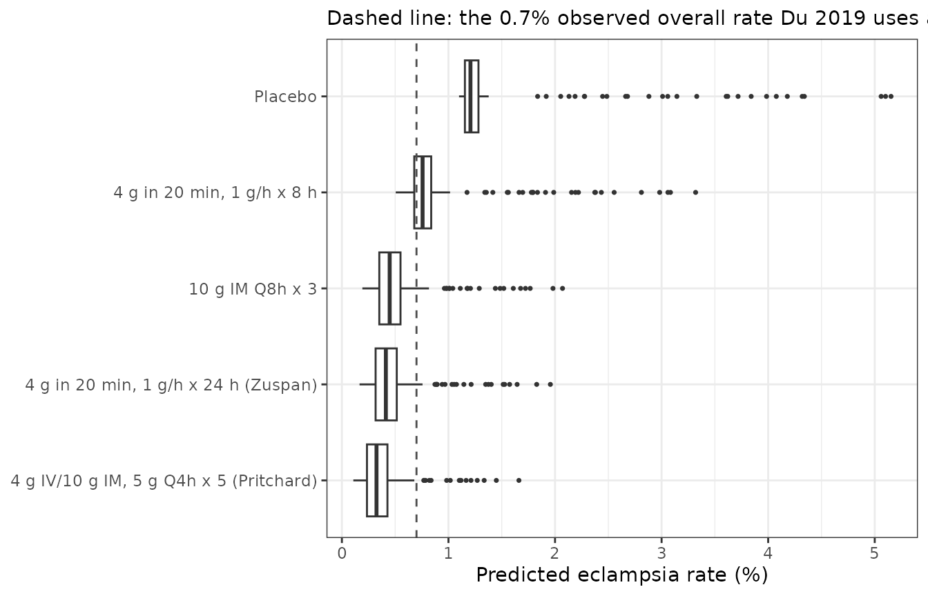

Per-woman predicted eclampsia rate in a 200-woman virtual cohort drawn from the Thai study covariate distributions.

cohort_summary <-
  cohort_out |>
  dplyr::group_by(regimen) |>
  dplyr::summarise(
    median_p = stats::median(p),
    q90_p = unname(stats::quantile(p, 0.90)),
    median_auc = stats::median(auc_mg),
    .groups = "drop"
  )

knitr::kable(cohort_summary, digits = 3,
             caption = "Virtual-cohort summary by regimen.")

Virtual-cohort summary by regimen.

regimen	median_p	q90_p	median_auc
10 g IM Q8h x 3	0.448	0.831	640.147
4 g IV/10 g IM, 5 g Q4h x 5 (Pritchard)	0.325	0.628	845.856
4 g in 20 min, 1 g/h x 24 h (Zuspan)	0.413	0.768	693.122
4 g in 20 min, 1 g/h x 8 h	0.757	1.572	297.052
Placebo	1.206	2.450	0.000

# Reference points for the exposure assertions below.
# (a) the AUC a Magpie woman gets under the Zuspan regimen, i.e. at the
#     imputed 85 kg / 0.8 mg/dL;
# (b) the AUC at the cohort's own median covariates;
# (c) the ratio of the cohort's median-covariate clearance to the typical
#     3.72 L/h, which is what sets the direction of the comparison.
auc_zuspan_ref <- magpie(28, 0)
med_cov <- data.frame(
  id = 1L, time = 0, amt = 0, evid = 0L,
  AGE = stats::median(cohort$AGE),
  WT = stats::median(cohort$WT),
  CREAT = stats::median(cohort$CREAT),
  DOSE_MGSO4_IV_G = 28, DOSE_MGSO4_IM_G = 0
)
med_cov_out <- as.data.frame(
  rxode2::rxSolve(mod, events = med_cov, returnType = "data.frame")
)
auc_median_covariate <- med_cov_out$auc_mg
cl_ratio <- med_cov_out$cl / 3.72

# The cohort is a random draw, so assert on the CENTRE and on a robust upper
# quantile -- never on the per-woman extreme, which moves with whichever
# subject happens to draw the smallest clearance.
stopifnot(
  # Risk is monotone decreasing in total effective dose.
  cohort_summary$median_p[cohort_summary$regimen == "Placebo"] >
    cohort_summary$median_p[cohort_summary$regimen == "4 g in 20 min, 1 g/h x 8 h"],
  cohort_summary$median_p[cohort_summary$regimen == "4 g in 20 min, 1 g/h x 8 h"] >
    cohort_summary$median_p[cohort_summary$regimen == "10 g IM Q8h x 3"],
  cohort_summary$median_p[cohort_summary$regimen == "10 g IM Q8h x 3"] >
    cohort_summary$median_p[cohort_summary$regimen == "4 g IV/10 g IM, 5 g Q4h x 5 (Pritchard)"],
  # Direction of the covariate effect on exposure. The cohort is both LIGHTER
  # (median WT below 85 kg, which lowers CL) and LESS RENALLY LOADED (median
  # creatinine below 0.8 mg/dL, which raises CL) than the 85 kg / 0.8 mg/dL
  # values Du 2019 imputed for the Magpie women. The creatinine term wins --
  # see cl_ratio below -- so the cohort's median AUC under a fixed 28 g must
  # sit BELOW the Magpie-imputed value, not above it.
  cl_ratio > 1,
  cohort_summary$median_auc[
    cohort_summary$regimen == "4 g in 20 min, 1 g/h x 24 h (Zuspan)"] <
    auc_zuspan_ref,
  # ... and not far below: the median of the cohort's AUC distribution agrees
  # with the deterministic solve at the cohort's median covariates to within
  # 5%, which is the Jensen-gap check for this nonlinear covariate function.
  abs(cohort_summary$median_auc[
    cohort_summary$regimen == "4 g in 20 min, 1 g/h x 24 h (Zuspan)"] /
    auc_median_covariate - 1) < 0.05,
  cohort_summary$median_auc[
    cohort_summary$regimen == "4 g in 20 min, 1 g/h x 24 h (Zuspan)"] >
    0.88 * auc_zuspan_ref,
  # Placebo carries no exposure at all.
  cohort_summary$median_auc[cohort_summary$regimen == "Placebo"] == 0,
  # Robust envelope rather than an extreme: even the 90th percentile of the
  # Pritchard arm stays under the 0.7% efficacy criterion.
  cohort_summary$q90_p[
    cohort_summary$regimen == "4 g IV/10 g IM, 5 g Q4h x 5 (Pritchard)"] < 0.7
)

The sampled cohort is more exposed per gram than the Magpie imputation would suggest in one respect and less in another, and the two do not cancel: its median serum creatinine of 0.66 mg/dL is below the 0.8 mg/dL reference, which raises clearance, while its median weight of 74.8 kg is below the 85 kg reference, which lowers it. The creatinine term wins by a margin – the net clearance at the cohort’s median covariates is 4% above the typical 3.72 L/h – so the same 28 g course delivers 693 mgh/L here against 742 mgh/L for an imputed Magpie woman. This is the mechanism behind Du 2019’s own recommendation that dose be individualised on body weight and serum creatinine.

Why there is no PKNCA section

PKNCA validates a concentration-time profile against published non-compartmental parameters. This model produces neither: it has no ODE state, no dose events and no time axis, and its only output is a probability. The exposure metric it consumes is an analytic AUC rather than a trapezoidal one, and it is checked directly against Du 2019’s reported median AUC values above. The published Cmax column of Table 1 is not reproducible from this model – see below.

Assumptions and deviations

• The Cmax column of Table 1 is out of scope. Table 1 reports a predicted peak magnesium concentration for each regimen alongside the eclampsia rate, and Du 2019 uses a 3.5 mmol/L threshold as its safety criterion. Reproducing it needs the full two-compartment disposition with intramuscular absorption. Supplemental Table S1 does give the disposition estimates (CL 3.72 L/h, Vc 15.4 L, Q 3.66 L/h, Vp 17.0 L, with IIV, inter-occasion variability on CL and a combined residual error), but the intramuscular absorption rate constant is not reported anywhere in this article or its supplement – the Limitations section says only that it used “absorption rate constant and absolute bioavailability values from the literature”, citing Salinger 2013. That model belongs to the companion publication doi:10.1002/jcph.1328 and is not shipped here. For a magnesium sulfate concentration-time model in this library see Salinger_2013_magnesiumSulfate, Easterling_2018_magnesium_sulfate or Deng_2024_magnesiumSulfate.
• The clearance parameters are fixed, not estimated here. lcl, e_creat_cl, e_wt_cl and lfdepot are wrapped in fixed() because Du 2019 carried them in from the companion population PK analysis as constants. Only the five logistic coefficients were estimated by this paper. No standard errors are reported for any of them.
• The published age branches are discontinuous at the knot and are encoded as printed rather than reconciled to the continuous form the Methods equation describes. See Model structure. The consequence for users: predictions for women near 22 years old should be treated with care, and the model should not be used to interpolate risk across that boundary.
• Doses are supplied as grams of MgSO4-7H2O, the administered salt. The conversion to elemental magnesium (0.098612 g Mg per g of the heptahydrate, from the atomic mass of magnesium over the formula mass of the salt) is done inside model(). Du 2019 states the relationship only as “contains ~10% of magnesium” in the Table 1 footnote; the exact stoichiometric value is used here because the approximate one does not reproduce Table 1 or the published AUC medians. Feeding this model doses expressed as elemental magnesium, or as anhydrous MgSO4, will silently give wrong answers.
• Both dose columns are whole-course totals, not per-administration amounts, and a woman can carry a non-zero value in both simultaneously (an intravenous loading dose followed by intramuscular maintenance).
• The placeholder residual is not from the source. addSd_prob_eclampsia = fixed(0.001) exists only so the nlmixr2 observation machinery accepts the model; Du 2019 fits an exact Bernoulli likelihood and estimates no residual error and no between-subject random effects. Read prob_eclampsia as a deterministic probability, and sample outcomes with rbinom(n, 1, prob_eclampsia) on the rxSolve() output if binary events are wanted.
• Two screened covariates carry no estimate. Preeclampsia severity (the blood-pressure / urinary-protein level) and previous anticonvulsant use were tested and not retained; no point estimate exists on disk. They are documented in covariatesDataExcluded rather than covariateData.
• The virtual cohort’s covariate distributions are an assumption. Du 2019 reports only means, SDs and the P5-P95 span per covariate (Table S3), not a correlation structure or a distributional family. The cohort above draws weight and creatinine independently from log-normals matched to the reported moments and age from a truncated normal; the real cohort’s weight and creatinine are almost certainly positively correlated, which would widen the clearance distribution relative to what is simulated here. This affects only the cohort section, not the Table 1 reproduction, which uses Du 2019’s own factorial grid.
• Extrapolation beyond the studied exposure range is not supported. The logit is linear and unbounded in AUC, so at AUC above roughly 2800 mgh/L the predicted rate falls below what any observation constrains, and Du 2019 reports that the model already under-predicts the observed rate in its lowest exposure quantile (0-371 mgh/L), attributing that to women who seized within 20 minutes of starting treatment.