SAR442257 trispecific T-cell engager QSP (Abrams 2022)
Source:vignettes/articles/Abrams_2022_sar442257_qsp.Rmd
Abrams_2022_sar442257_qsp.Rmd
# The model has 773 ODE states, so building the rxode2 UI takes about a
# minute and the first solve compiles it (about another minute). Build it once
# and reuse it throughout.
ui <- rxode2::rxode2(readModelDb("Abrams_2022_sar442257_qsp"))
Model and source
- Citation: Abrams RE, Pierre K, El-Murr N, Seung E, Wu L, Luna E, Mehta R, Li J, Larabi K, Ahmed M, Pelekanou V, Yang ZY, van de Velde H, Stamatelos SK. Quantitative systems pharmacology modeling sheds light into the dose response relationship of a trispecific T cell engager in multiple myeloma. Sci Rep. 2022;12:10976. doi:10.1038/s41598-022-14726-5
- Description: In vitro (human peripheral-blood T cells, CD38+ PBMCs and multiple myeloma cells). QSP. Rule-based quantitative systems pharmacology model of the CD38xCD28xCD3 trispecific T-cell engager SAR442257 in multiple myeloma: the dose-prediction form of the in vitro model (760 species plus 13 cumulative flux trackers, 773 ODE states). Naive, effector memory and active CD4+ and CD8+ T cells, multiple myeloma (MM) cells, a lumped CD38+ PBMC population and shed soluble CD38 bind free drug through the CD3, CD28 and CD38 arms; any pair of cells whose arms can be bridged by drug forms a synapse with a collision-driven rate (Figure 1C). Effector memory cells activate in a CD3-arm synapse at a constant rate; naive cells need drug on both CD3 and CD28 (a Michaelis-Menten AND gate). Active T cells proliferate and kill MM cells and PBMCs in synapse, T cell-MM synapses become killing-resistant, and active T cells and synapsed PBMCs/MM cells release IFN-gamma, TNF-alpha, IL-6 and IL-10 (outputs only). Deterministic mechanism model with no IIV and no error model. Drug is dosed as molecules into tsAb (1 nM is Vol * 6.022e14 molecules); setting kon_CD28 = 0 gives the comparator CD38xCD3 bispecific.
- Article: https://doi.org/10.1038/s41598-022-14726-5
- Supplement (Matlab model-generation code, Tables S1-S2, Figures S1-S9): https://www.nature.com/articles/s41598-022-14726-5 (Supplementary Information)
SAR442257 is the CD38xCD28xCD3 trispecific T-cell engager described by Wu et al. (Nature Cancer 2020); the paper refers to it as the CD38xCD28xCD3 tsAb and names its first-in-human trial, NCT04401020, whose registered intervention is SAR442257.
Population
This is an in vitro model, not a population model. It was calibrated in three stages: T-cell activation in PBMCs, killing of the RPMI-8226 (CD38 high) and KMS-11 (CD38 low) myeloma lines by pre-activated CD8+ T cells, and cytokine release in the MIMIC assay. The packaged parameter set is the dose-prediction module in Table S2. It represents a peripheral-blood sample from a multiple myeloma patient: 39,177 T cells (naive, effector memory and active CD4+ and CD8+), 3,920 MM cells and 29,000 CD38+ PBMCs, with soluble CD38 at 4.96e6 molecules. The paper simulates the module for 72 h at fixed drug concentrations from 8.4e-4 nM (the MABEL dose) to 0.672 nM (Figure 3).
The paper also builds an “in vitro population” by sampling around the MIMIC calibration (Figure 2D) and reports some results as that population’s mean and SD (Figure 4C). That population is not deposited, so this file carries only the single parameter set of Table S2. Figure 3 uses “one set of values from the final population”, and the simulations below reproduce it.
How the equations were obtained
The paper deposits its Matlab model-generation code rather than the
equations. The ODEs here were produced by running that code unchanged
(Supplementary MOESM1-3; main script with
Nm = 'tsAb_FullODEs_DosePred'). The run gave the 760
species and 13 flux trackers the paper describes. The resulting
tsAb_FullODEs_DosePred_Original.m was then translated term
by term: X(idx.<name>) became the state
<name> and ps.<name> became the
parameter <name>. The state names are the generator’s
own:
-
CD8_N,CD8_EM,CD8_A,CD4_N,CD4_EM,CD4_A,MM,TRGT: free cells. -
R_<cell>_<receptor>andR_<cell>_<receptor>_tsAb: free and drug-bound receptors on free cells. -
S_<cell1>_<arm1>_<cell2>_<arm2>: a synapse betweencell1, engaged through drug armarm1, andcell2, engaged througharm2._MUTmarks a killing-resistant synapse. -
S_..._BrandS_..._R_<cell>_<receptor>[_tsAb]: the drug bridges and the receptors held inside each synapse. -
IFNg,TNFa,IL6,IL10,sCD38: soluble species. -
TcellSyn…SynFormation: the generator’s cumulative flux trackers.
The generator inlines the synapse-formation flux (Figure 1C), the two
bridge formation terms and the naive-cell activation rate at every point
of use. The packaged model computes each of these once per synapse
instead (kf_*, kb1_*, kb2_*,
ka_*). Before shipping, the maintainers compiled the fully
inlined and the factored systems side by side. At 0, 8.4e-3 and 0.672 nM
the two gave identical solutions for all 773 states (maximum relative
difference 0). The inlined form is not compiled here because it doubles
the build time.
Source trace
| Model element | Source |
|---|---|
| Species list, synapse combinations, killing / resistance / dissociation / activation assignments | Supplementary MOESM1 (DefineSpecified_2cellSyn), MOESM3
(Receptors_Def_perCell) |
| Assembly of every ODE term, flux trackers | Supplementary MOESM2 (main generation script) |
Synapse-formation template kf_*, including bridge
dissociation koffR1 + koffR2
|
Figure 1C; MOESM2 konOFF_Cell
|
Naive activation AND gate ka_*, EM activation
kact_EM
|
Methods, “Model equations”; MOESM1 ActRt_2cell
|
Killing (kkillMM_*, kkillTRGT_*),
resistance (kmut_SYN), synapse dissociation
(kDis) |
Table S2; MOESM1 |
Cell lifecycle (ksyn_*, kdeg_*,
kpr_*, C_M_MM) |
Table S2 |
Drug binding (kon_*, koff_*), well volume
(Vol) |
Table S2 |
Antigen densities (CD3per_*, CD28per_*,
CD38per_*) |
Table S2 |
Collision factor, bridges per synapse, scaling cell numbers
(kcoll, Br_perS,
<cell>_0) |
Table S2 |
Cytokine production and degradation (kprod_*,
kdeg_<cytokine>) |
Table S2; Methods, “Model overview” |
Soluble CD38 (kshedMM_s38, kshedTRGT_s38,
kdeg_sCD38) |
Table S2 |
Initial cell numbers and soluble CD38 (bl_*) |
Table S2, “Initial Value” block |
Ineffective-synapse definition used in mm_ineff
|
Generator output file tsAb_FullODEs_DosePred_SYNie
(SYN_MMiec); Methods, bispecific paragraph |
Bispecific comparator (kon_CD28 = 0) |
Methods, “Model simulation” |
Each ini() line in the model file names its Table S2
row.
Simulation of the dose-prediction module (Figure 3)
The paper simulates fixed drug concentrations added at time zero (a
constant amount of drug that is cleared only through killing of target
cells and dissociation of synapses). The dose is entered as molecules in
the well: nM * Vol * 6.022e14.
nM_to_molecules <- 2.00e-4 * 6.02214076e14 # Table S2 Vol (L) x Avogadro x 1e-9
doses_nM <- c(0, 8.4e-4, 2.52e-3, 8.4e-3, 2.1e-2, 4.2e-2, 8.4e-2, 0.168, 0.252, 0.336, 0.504, 0.672)
obs_times <- seq(0, 72, by = 2)

events <- bind_rows(lapply(seq_along(doses_nM), function(i) {
  data.frame(
    id = i,
    time = c(0, obs_times),
    evid = c(1L, rep(0L, length(obs_times))),
    amt = c(doses_nM[i] * nM_to_molecules, rep(0, length(obs_times))),
    cmt = "tsAb"
  )
}))
dose_key <- data.frame(id = seq_along(doses_nM), dose_nM = doses_nM)
# Loose-but-adequate tolerances: atol 1e-4 is far below one cell or one
# molecule, and the 72-h endpoints below agree to 0.1 percentage point with a
# solve at atol = rtol = 1e-8.
sim_tri <- rxSolve(ui, events, atol = 1e-4, rtol = 1e-5, maxsteps = 1e6, returnType = "data.frame")
cell_states <- ui$state
sim_tri <- left_join(sim_tri, dose_key, by = "id")
fig3 <- sim_tri |>
  select(time, dose_nM, pct_mm_killed, tact_total, tact_free, pct_mm_ineff) |>
  pivot_longer(-c(time, dose_nM)) |>
  mutate(name = factor(name,
    levels = c("pct_mm_killed", "tact_total", "tact_free", "pct_mm_ineff"),
    labels = c(
      "A. MM cell killing (%)", "B. Activated T cells (#)",
      "C. Free active T cells (#)", "D. Ineffective MM synapses (% original MM)"
    )
  ))
ggplot(fig3, aes(time, value, colour = factor(signif(dose_nM, 3)))) +
  geom_line() +
  facet_wrap(~name, scales = "free_y") +
  labs(x = "Time (h)", y = NULL, colour = "Dose (nM)") +
  theme_bw()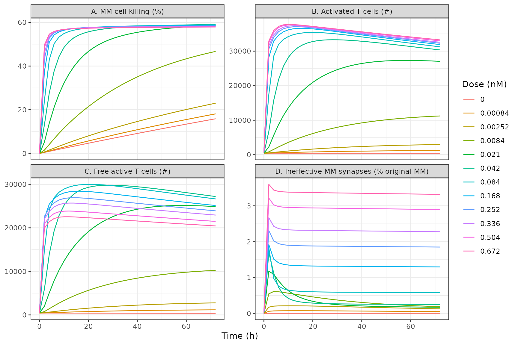
Replicates Figure 3A-D of Abrams 2022: MM killing, total and free active T cells, and ineffective MM synapses over 72 h for each fixed drug concentration.
Values at 72 h compared with the curve end-points the maintainers read off Figure 3A and 3D:
published_72h <- data.frame(
  dose_nM = doses_nM,
  kill_published = c(15.6, 18.0, 22.9, 46.6, 58.6, 59, 59, 58.5, 58.5, 58, 58, 58),
  ineff_published = c(NA, NA, NA, NA, NA, NA, 0.57, 1.28, 1.85, 2.28, 2.90, 3.32)
)
end72 <- sim_tri |>
  filter(time == 72) |>
  select(dose_nM, pct_mm_killed, pct_mm_ineff, tact_total, tact_free) |>
  left_join(published_72h, by = "dose_nM")
end72 |>
  transmute(
    "Dose (nM)" = signif(dose_nM, 3),
    "Killing, simulated (%)" = round(pct_mm_killed, 1),
    "Killing, Figure 3A (%)" = kill_published,
    "Ineffective synapses, simulated (%)" = round(pct_mm_ineff, 2),
    "Ineffective synapses, Figure 3D (%)" = ineff_published,
    "Total active T cells" = round(tact_total),
    "Free active T cells" = round(tact_free)
  ) |>
knitr::kable()| Dose (nM) | Killing, simulated (%) | Killing, Figure 3A (%) | Ineffective synapses, simulated (%) | Ineffective synapses, Figure 3D (%) | Total active T cells | Free active T cells |
|---|---|---|---|---|---|---|
| 0.00000 | 15.9 | 15.6 | 0.00 | NA | 365 | 365 |
| 0.00084 | 18.1 | 18.0 | 0.05 | NA | 1224 | 1175 |
| 0.00252 | 23.0 | 22.9 | 0.13 | NA | 2945 | 2772 |
| 0.00840 | 46.7 | 46.6 | 0.19 | NA | 11225 | 10240 |
| 0.02100 | 58.6 | 58.6 | 0.17 | NA | 27034 | 24879 |
| 0.04200 | 59.0 | 59.0 | 0.25 | NA | 30338 | 27188 |
| 0.08400 | 58.9 | 59.0 | 0.58 | 0.57 | 31242 | 26642 |
| 0.16800 | 58.6 | 58.5 | 1.30 | 1.28 | 31895 | 25124 |
| 0.25200 | 58.4 | 58.5 | 1.85 | 1.85 | 32284 | 23904 |
| 0.33600 | 58.2 | 58.0 | 2.28 | 2.28 | 32569 | 22932 |
| 0.50400 | 58.0 | 58.0 | 2.90 | 2.90 | 32975 | 21479 |
| 0.67200 | 57.9 | 58.0 | 3.32 | 3.32 | 33258 | 20441 |
# Deterministic model: there is no cohort, so these differences are the
# reading precision of the published figure and nothing else. 2 percentage
# points of killing and 0.15 of ineffective synapses is about the line width.
stopifnot(
  all(abs(end72$pct_mm_killed - end72$kill_published) < 2),
  all(abs(end72$pct_mm_ineff - end72$ineff_published) < 0.15, na.rm = TRUE),
  # Figure 3B / 3C at 0.672 nM: about 3.3e4 total and 2.05e4 free active
  # T cells at 72 h, total peaking near 3.75e4.
  abs(end72$tact_total[end72$dose_nM == 0.672] / 3.3e4 - 1) < 0.05,
  abs(end72$tact_free[end72$dose_nM == 0.672] / 2.05e4 - 1) < 0.05,
  abs(max(sim_tri$tact_total) / 3.75e4 - 1) < 0.05
)
Without drug the simulated killing at 72 h is 15.9%. This is net
natural loss alone: 1 - exp(-(kdeg_MM - kpr_MM) * 72) =
15.9% with Table S2’s kdeg_MM = 0.0025 and
kpr_MM = 1e-4 1/h. So the paper’s “MM cell killing” is loss
from the initial MM count, not killing relative to an untreated control,
and pct_mm_killed is defined the same way.
Flux balance (Figure 1D)
The generator tracks cumulative cell creation and destruction in its flux states. The paper checks that the total cell count always equals the initial count plus the net flux (Figure 1D). The same check on the packaged model, for MM cells and CD38+ PBMCs at the two doses shown in Figure 1D, follows. The two sides come from one solve, so they should differ only by integration error.
synapse_states <- grep("^S_", cell_states, value = TRUE)
synapse_states <- synapse_states[!grepl("_R_|_Br$", synapse_states)]
# Number of CD38+ PBMCs held in each synapse species (0 or 1).
trgt_mult <- lengths(regmatches(paste0(synapse_states, "_"), gregexpr("_TRGT_", paste0(synapse_states, "_"))))
fb <- sim_tri |>
  filter(dose_nM %in% c(8.4e-4, 0.672)) |>
  mutate(
    trgt_total = TRGT + as.numeric(as.matrix(pick(all_of(synapse_states))) %*% trgt_mult),
    mm_balance = 3.92e3 + MMcellSyn - MMcellDeg,
    trgt_balance = 2.90e4 + TRGTcellSyn - TRGTcellDeg
  )
fb |>
  filter(time %in% c(0, 24, 72)) |>
  transmute(
    "Dose (nM)" = dose_nM, "Time (h)" = time,
    "MM total" = round(mm_total, 2), "MM initial + net flux" = round(mm_balance, 2),
    "PBMC total" = round(trgt_total, 1), "PBMC initial + net flux" = round(trgt_balance, 1)
  ) |>
knitr::kable()| Dose (nM) | Time (h) | MM total | MM initial + net flux | PBMC total | PBMC initial + net flux |
|---|---|---|---|---|---|
| 0.00084 | 0 | 3920.00 | 3920.00 | 29000.0 | 29000.0 |
| 0.00084 | 24 | 3653.66 | 3653.66 | 26600.1 | 26600.1 |
| 0.00084 | 72 | 3209.89 | 3209.89 | 22379.5 | 22379.5 |
| 0.67200 | 0 | 3920.00 | 3920.00 | 29000.0 | 29000.0 |
| 0.67200 | 24 | 1670.09 | 1670.09 | 26733.9 | 26733.9 |
| 0.67200 | 72 | 1651.39 | 1651.39 | 22712.8 | 22712.8 |
Trispecific versus bispecific (Figure 4C)
The paper simulates the comparator CD38xCD3 bispecific by setting
kon_CD28 to 0 and nothing else. Figure 4C plots 72-h
killing against an unlabelled “dose low -> high” axis as the mean and
SD of the unpublished in vitro population. The single Table S2 parameter
set can therefore be compared with the shape of that figure but not with
its values.
sim_bi <- rxSolve(ui, events,
  params = c(kon_CD28 = 0),
  atol = 1e-4, rtol = 1e-5, maxsteps = 1e6, returnType = "data.frame"
) |>
  left_join(dose_key, by = "id")
fig4c <- bind_rows(
  sim_tri |> filter(time == 72) |> mutate(molecule = "Trispecific"),
  sim_bi |> filter(time == 72) |> mutate(molecule = "Bispecific (kon_CD28 = 0)")
) |>
  filter(dose_nM > 0)
ggplot(fig4c, aes(dose_nM, pct_mm_killed, colour = molecule)) +
  geom_line() +
  geom_point() +
  scale_x_log10() +
  labs(x = "Dose (nM)", y = "MM killing at 72 h (%)", colour = NULL) +
  theme_bw()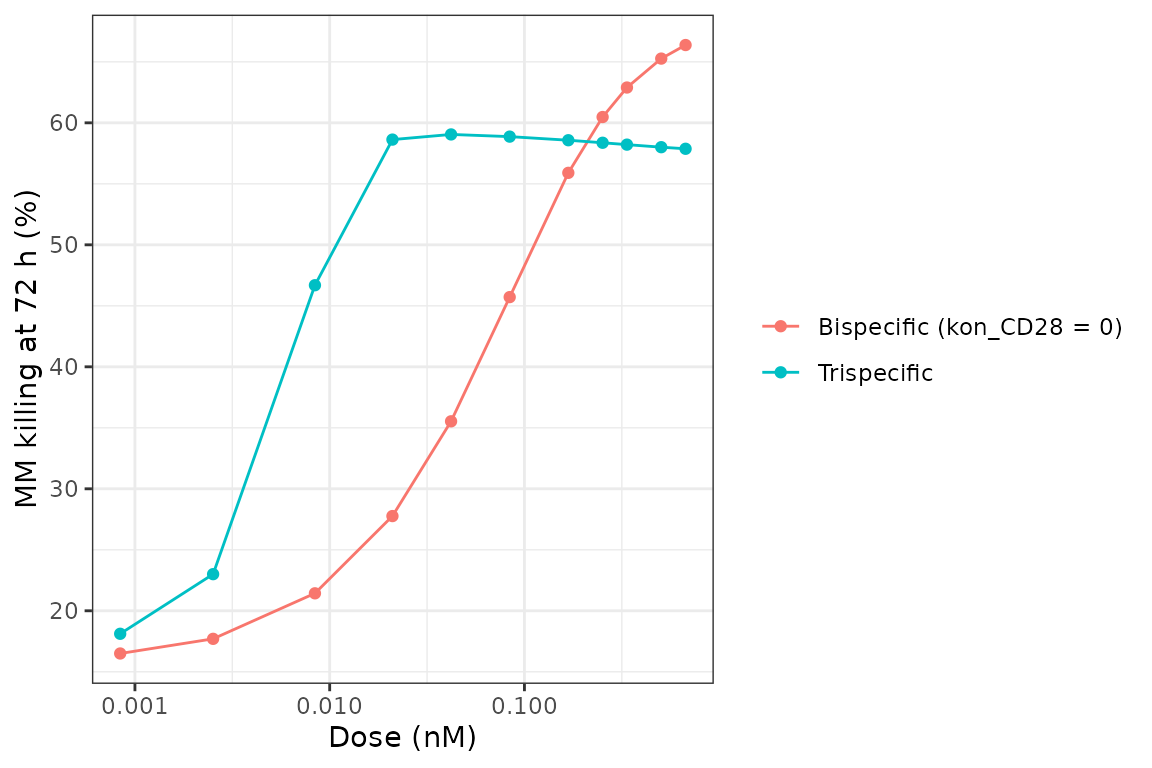
Replicates the shape of Figure 4C of Abrams 2022: 72-h MM killing for the trispecific and the CD28-null bispecific across the Figure 3 dose grid (single Table S2 parameter set, not the population mean).
fig4c |>
  select(dose_nM, molecule, pct_mm_killed) |>
  pivot_wider(names_from = molecule, values_from = pct_mm_killed) |>
  mutate(across(-dose_nM, \(x) round(x, 1)), dose_nM = signif(dose_nM, 3)) |>
  rename("Dose (nM)" = dose_nM) |>
knitr::kable()| Dose (nM) | Trispecific | Bispecific (kon_CD28 = 0) |
|---|---|---|
| 0.00084 | 18.1 | 16.5 |
| 0.00252 | 23.0 | 17.7 |
| 0.00840 | 46.7 | 21.4 |
| 0.02100 | 58.6 | 27.8 |
| 0.04200 | 59.0 | 35.5 |
| 0.08400 | 58.9 | 45.7 |
| 0.16800 | 58.6 | 55.9 |
| 0.25200 | 58.4 | 60.5 |
| 0.33600 | 58.2 | 62.9 |
| 0.50400 | 58.0 | 65.3 |
| 0.67200 | 57.9 | 66.4 |
tri72 <- fig4c$pct_mm_killed[fig4c$molecule == "Trispecific"]
bi72 <- fig4c$pct_mm_killed[fig4c$molecule != "Trispecific"]
# Results text: "The largest difference was in the low doses when the
# trispecific antibody killing was up to threefold increase from the
# bispecific antibody", and "At higher drug doses ... slightly higher
# bispecific killing for these doses". Deterministic model, so both
# margins are wide (a 2.1-fold low-dose ratio and an 8.5-point high-dose
# lead in this solve).
stopifnot(
  max(tri72 / bi72) > 1.5,
  bi72[length(bi72)] > tri72[length(tri72)] + 4
)
The single parameter set reproduces the shape of Figure 4C. The trispecific advantage is largest at the low doses: at 2.1e-2 nM the trispecific kills 2.1 times as many MM cells as the bispecific (the paper: “up to threefold”). Here the CD28 arm both costimulates naive T cells and lets MM cells join synapses through CD28. The trispecific plateaus near 58% from about 2e-2 nM upwards. The bispecific keeps rising and overtakes it at 0.25 nM and above, reaching 66.4% at 0.672 nM; Figure 4C shows about 67% against about 60%. The descending limb of the bispecific’s bell-shaped curve lies beyond the top of the Figure 3 dose grid simulated here. Because Figure 4C’s dose axis is unlabelled, that limb is not checked.
Assumptions and deviations
-
Bridge dissociation rate. The generator multiplies
the bridge term by
koffc_<receptor>, which Table S2 does not list. Figure 1C writes the same term as(koffR1 + koffR2) * BR_SYNwith the drug-receptor dissociation rates, and the Methods describe bridge formation with the “typical kon/koff formulation”.koffc_<R>is therefore set equal tokoff_<R>. The Figure 3 reproduction above, including the 3.32% ineffective synapses at 0.672 nM, supports this. -
Cytokine production by naive and effector memory T
cells. The generator references
kprod_<CD4|CD8>_<N|EM>_<cytokine>, which Table S2 does not list. They are set to zero because the Methods state that “active T-cells produce TNF-alpha, IFN-gamma, and IL-6”. Cytokines are outputs only and do not feed back on any other state. -
MM-cell cytokine production. Table S2 gives the MM
rates as “Assume same as TRGT rates” with no value. The model uses the
kprod_TRGT_*parameters in place ofkprod_MM_*. -
CD38+ PBMC proliferation. Table S2 sets
kpr_TRGT = 0, so the generator’s logistic termkpr_TRGT * (1 - TRGT / C_M_TRGT) * TRGTis zero. The term is omitted, because its carrying capacityC_M_TRGTis not reported. -
Dosing. The generator adds a constant input
ps.Doseto the drug equation. The Methods describe drug added at a fixed level and cleared only by killing and synapse dissociation, so doses here are entered as an amount at time zero. Users can still give an infusion throughrateontsAb. The nM-to-molecule conversion uses the Table S2 well volumeVol = 2e-4L, which also makes the per-moleculekonvalues physically sensible (kon_CD38 = 1.36e-11per molecule per hour is 4.6e5 per molar per second). The Figure 3 reproduction confirms both choices. -
Soluble CD38 at time zero. The Methods say sCD38
“is not present initially” in the in vitro model. However, Table S2
gives an initial value of 4.96e6 molecules for the dose-prediction
module, citing a literature serum level. The Table S2 value is used
because this file is the dose-prediction module, and each soluble CD38
molecule starts with one free CD38 site. Set
bl_sCD38 = 0for the calibration-experiment setting. -
Scaling cell numbers. Table S2 describes the
<cell>_0constants in the synapse-formation denominator as “Set to initial cell number”. However, the printed values do not equal the printed initial cell numbers: for example,MM_0 = 2540800against an initial 3,920 MM cells. Presumably they come from the experiment in whichkcollwas calibrated. They are used as printed; with them the Figure 3 curves are reproduced. - No variability. The paper’s in vitro population is not published. The model carries no IIV and no residual error. Figure 2 (calibration fits) and the population means and SDs in Figure 4C are not reproduced; only the shape of Figure 4C is compared.
-
Units.
kshedMM_s38is printed in “Molecules/cell/hr”, but the generator multiplies it by the number of free MM-cell CD38 receptors, so it acts per receptor (1/h). The label states this.