Model and source
#> ℹ parameter labels from comments will be replaced by 'label()'Citation: Lee A, Liu C, Tran MT, Phal S, Peloquin CA, Nieves D, Capparelli E, Arrieta AC. Population pharmacokinetics and safety of continuous oxacillin in preterm and term neonates and infants. Antimicrob Agents Chemother. 2026;70(6):e01777-25. doi:10.1128/aac.01777-25.
Description: One-compartment intravenous population pharmacokinetic model with first-order elimination for oxacillin in 22 preterm and term neonates and infants aged 4 to 82 days postnatal (gestational age 23.9 to 40.3 weeks), each given a 25 mg/kg loading dose over 30 min followed immediately by a continuous infusion of 160 mg/kg/day (120 mg/kg/day for the single infant born at <32 weeks gestation and enrolled at <14 days of life), with 79 evaluable plasma concentrations fitted in NONMEM 7.5.0 by FOCE-I (ADVAN1 TRANS2). Clearance carries a fixed allometric weight exponent of 0.75 and an estimated power effect of postnatal age (exponent 0.433), both normalised to the typical infant of 3.4 kg and 36 days; central volume is linear in weight over the same 3.4 kg reference. Postnatal age was the only covariate retained: gestational age, postmenstrual age, height, body surface area, albumin, serum creatinine and baseline transaminases were screened and rejected, and they are recorded in covariatesDataExcluded rather than in the model. Between-subject variability could only be estimated for clearance. Oxacillin is dosed directly into
central. The unbound concentration Cu that drives the paper’s fT > MIC target-attainment analysis is derived algebraically as 10% of the total concentration, an unbound fraction the authors fixed from the literature rather than measuring. The magnitudes of the combined additive-plus-proportional residual error are not reported anywhere in the paper or its supplements, so both residual standard deviations are encoded as fixed(0); see the vignette Errata.Article: https://doi.org/10.1128/aac.01777-25 (open access, CC BY 4.0)
Supplement: Table S1 (adverse events), Table S2 (raw per-patient data), Table S3 (raw concentrations), published with the open-access article (PMC13231926).
Oxacillin is the standard-of-care antistaphylococcal penicillin for
methicillin-susceptible Staphylococcus aureus, but before this
study no pharmacokinetic data existed in neonates and young infants. Lee
2026 is a prospective phase 1 study in 22 infants at most 90 days old,
each given a 25 mg/kg loading dose over 30 min followed immediately by a
continuous infusion. The paper’s clinical question is whether the
unbound concentration stays above the MIC for the whole dosing exposure
(fT 100% > MIC), which for a continuous infusion reduces
to whether the steady-state unbound concentration exceeds the MIC.
Population
| Field | Value |
|---|---|
| species | human |
| n_subjects | 22 |
| n_studies | 1 |
| n_observations | 79 |
| age_range | 4-82 days postnatal (inclusion criteria >3 to <=90 days) |
| age_median | 32 days postnatal (IQR 12-46) |
| ga_range | 23.9-40.3 weeks gestational age at birth |
| ga_median | 38 weeks (IQR 30-39) |
| weight_range | 0.605-7.025 kg |
| weight_median | 3.29 kg |
| sex_female_pct | 27 |
| race_ethnicity | Hispanic 73%; White 14%; Black 5%; Hispanic/Black 5%; Hispanic/White 5% |
| disease_state | Hospitalized neonates and young infants receiving oxacillin as standard of care: 11 empiric therapy for suspected infection, 9 confirmed methicillin-susceptible Staphylococcus aureus infection (osteomyelitis n = 1, pneumonia n = 3, bacteraemia n = 3, skin/soft tissue n = 2), 1 methicillin-susceptible S. epidermidis bacteraemia, 1 perioperative prophylaxis. Critically ill infants could not be enrolled, and renal dysfunction (dialysis, urine output <0.5 mL/kg/h, or serum creatinine >1.7 mg/dL), transaminases >5x ULN, therapeutic hypothermia within 24 h and ECMO were exclusion criteria, so the model should not be extrapolated to those states. |
| dose_range | 25 mg/kg intravenous loading dose over 30 min, immediately followed by a continuous intravenous infusion of 160 mg/kg/day (21 of 22 infants) or 120 mg/kg/day (1 infant in Cohort 4: gestational age <32 weeks and postnatal age <14 days) |
| sampling | Convenience sampling, maximum five samples per infant (minimum 25 uL each): a baseline sample before the loading dose and then 30-120 min, 8-16 h and 16-96 h after the start of the continuous infusion, plus one within 1 h after the end of infusion. Group 1 and four further infants had at most three samples to limit phlebotomy. Of 89 plasma samples, 10 were below the 2 mcg/mL lower limit of quantification (9 of them baseline) and were excluded, leaving 79. Plasma assayed by validated LC-MS/MS at the University of Florida Infectious Disease Pharmacokinetics Laboratory over a 2-100 mcg/mL calibration range with within- and between-day CV <10%. One cerebrospinal-fluid concentration was collected and was NOT included in the final model. |
| regions | United States (single centre, Children’s Hospital of Orange County, California) |
| notes | Prospective, phase 1, open-label, single-centre study. Demographics are Lee 2026 Table 1; per-patient raw values are Supplemental Table S2. Enrolment was stratified into four cohorts by gestational age (<32 vs >=32 weeks) and postnatal age (<14 vs >=14 days) targeting 6 infants each, but Cohort 4 (GA <32 weeks, PNA <14 days) recruited only 1 of 6. Model reliability was assessed by 1,000-set bootstrapping in Wings for NONMEM; every final estimate fell inside its bootstrap 95% confidence interval. eta-shrinkage on clearance was 8.27%. Table 1’s total male count (15, 68%) disagrees with the sum of its own per-cohort entries (8 + 3 + 4 + 1 = 16) and with Supplemental Table S2, which lists 16 male and 6 female infants; the 27% female recorded here follows the raw data. Median measured total oxacillin concentration 20.2 mcg/mL (IQR 11.8-36.2). Safety: 45 adverse events in 18 infants, 12 possibly oxacillin-related, 3 serious events none of them related, no deaths. |
Twenty-two infants completed the study (Lee 2026 Table 1). Gestational age at birth ranged from 23.9 to 40.3 weeks (median 38) and postnatal age at enrolment from 4 to 82 days (median 32). Weights, which Table 1 does not tabulate, are in Supplemental Table S2 and span 0.605 to 7.025 kg with a median of 3.29 kg. Enrolment was stratified into four cohorts by gestational age (<32 vs >=32 weeks) and postnatal age (<14 vs >=14 days) targeting six infants each; the preterm-and-youngest cohort recruited only one of six, which is why the paper declines to draw conclusions about gestational age. Twenty-one infants received 160 mg/kg/day by continuous infusion and one received 120 mg/kg/day. Of 89 plasma samples 10 were below the 2 mcg/mL limit of quantification and were excluded, leaving 79 concentrations for the fit.
The same information is available programmatically via
readModelDb("Lee_2026_oxacillin")()$population.
Source trace
| Equation / parameter | Value | Source location |
|---|---|---|
lcl (CL for 3.4 kg, 36 d) |
1.01 L/h | Table 2, CL (Theta1); bootstrap 95% CI 0.791-1.3 |
lvc (V for 3.4 kg) |
1.87 L | Table 2, V (Theta2); bootstrap 95% CI 1.07-2.61 |
e_pna_cl |
0.433 | Table 2, Effect of PNA on CL (Theta3); bootstrap 95% CI
0.133-0.709 |
e_wt_cl |
0.75 (fixed) | Table 2 footnote b (WT_Kg/3.4)^0.75; Methods states CL
“was allometrically scaled by weight” – a-priori value, no estimate or
interval reported |
e_wt_vc |
1 (fixed) | Table 2 footnote b Vd = 1.87 * WT_Kg/3.4, i.e. linear
in weight |
etalcl |
0.568 read as a log-scale SD; variance 0.322624 | Table 2, IIV CL (etaCL); scale resolved below, not
stated in the paper |
fu |
0.1 (fixed) | Methods, “Simulations and pharmacodynamic assessments”: free concentrations “estimated at 10% of total concentrations as reported in the literature (9)” |
addSd, propSd
|
0 (fixed) | Methods declares “a combined additive and proportional within-subject error model”; no magnitude is reported anywhere in the paper or its supplements |
d/dt(central) <- -kel * central |
n/a | Results, “Pharmacokinetic model”: one-compartment, first-order elimination, NONMEM ADVAN1 TRANS2 |
| Reference weight 3.4 kg, reference PNA 36 d | n/a | Table 2 footnote b, and Results, “a typical infant 36 days postnatal age and weighing 3.4 kg” |
Reading the published between-subject variability
Table 2 prints IIV CL (etaCL) = 0.568 with no unit and
no variance / SD / CV qualifier. Read as a NONMEM $OMEGA
variance it implies a log-scale SD of
sqrt(0.568) = 0.754; read as a standard
deviation it is 0.568 itself. The two readings differ by a
third in spread and change every target-attainment number in the paper,
so the choice cannot be left implicit. Two independent checks against
the paper’s own data both exclude the variance reading.
Check 1 – individual clearances recovered from Supplemental Table S2
Under a continuous infusion the steady-state concentration is exactly
rate / CL, so each infant’s clearance is recoverable from
the supplement without any fitting. The table below transcribes, for all
22 infants, Supplemental Table S2’s current weight, dose-calculating
weight, postnatal age, daily dose and the two on-infusion samples (the
8-16 h and 16-96 h windows, both at or beyond the ~5 half-lives needed
for steady state).
s2 <- tibble::tribble(
  ~id,     ~wt,  ~dwt, ~pna, ~dose,     ~c2,   ~t2,     ~c3,   ~t3,
  "Pt1",  1.605, 1.605,   82,   160,  62.536, 10.07,  35.859, 81.07,
  "Pt3",  4.155, 4.155,   39,   160,  10.667, 10.38,  12.390, 30.15,
  "Pt4",  3.500, 3.500,   34,   160,  16.698,  8.67,   7.895, 69.70,
  "Pt5",  1.130, 1.130,   36,   160,      NA,    NA,   7.415, 16.93,
  "Pt6",  2.310, 2.000,    4,   160,      NA,    NA,  85.019, 17.00,
  "Pt8",  3.520, 3.515,   79,   160,  30.035, 14.88,  11.513, 35.35,
  "Pt9",  1.780, 1.785,   29,   160,      NA,    NA,  13.754, 46.87,
  "Pt11", 4.755, 3.170,   82,   160,  15.809,  8.57,  15.014, 18.13,
  "Pt12", 2.105, 2.105,   52,   160,      NA,    NA,  18.174, 39.08,
  "Pt14", 2.450, 2.500,    7,   160,  27.473, 11.20,  24.390, 35.28,
  "Pt16", 3.530, 3.530,    4,   160, 109.124,  8.28, 112.986, 16.43,
  "Pt17", 3.260, 3.260,   14,   160,   6.243,  8.15,  42.613, 44.93,
  "Pt18", 5.345, 5.345,   47,   160,  15.529, 11.10,  13.216, 17.67,
  "Pt21", 3.290, 3.290,   22,   160,  19.628, 11.70,  11.836, 16.57,
  "Pt22", 3.290, 3.290,   11,   160,  49.128,  9.08,  26.448, 17.55,
  "Pt23", 2.880, 2.880,   11,   160,  10.452, 12.38,  14.164, 63.35,
  "Pt24", 3.390, 3.390,   42,   160,  15.892,  8.75,  14.924, 16.23,
  "Pt25", 0.605, 0.697,    5,   120,      NA,    NA,  34.128, 16.00,
  "Pt26", 2.975, 2.975,   18,   160,  94.543,  9.08,  28.456, 59.58,
  "Pt27", 3.545, 3.500,   31,   160,  13.469, 12.63,  12.254, 17.52,
  "Pt28", 4.480, 4.480,   32,   160,  26.004,  8.35,  25.228, 16.60,
  "Pt29", 7.025, 7.025,   69,   160,  24.357,  9.20,   8.317, 15.88
)
stopifnot(nrow(s2) == 22L)

# Published covariate model, hard-coded from Table 2 footnote b so that this
# check is INDEPENDENT of what the model file happens to contain.
cl_published <- function(wt, pna_days) 1.01 * (wt / 3.4)^0.75 * (pna_days / 36)^0.433

s2 <- s2 |>
  mutate(
    rate   = dose * dwt / 24,             # mg/h delivered by the continuous infusion
    clpred = cl_published(wt, pna),
    eta2   = log((rate / c2) / clpred),   # log(CL_observed / CL_predicted)
    eta3   = log((rate / c3) / clpred),
    etabar = rowMeans(cbind(eta2, eta3), na.rm = TRUE)
  )

spread <- c(
  `16-96 h sample`   = sd(s2$eta3, na.rm = TRUE),
  `8-16 h sample`    = sd(s2$eta2, na.rm = TRUE),
  `per-infant mean`  = sd(s2$etabar)
)
round(spread, 3)
#>  16-96 h sample   8-16 h sample per-infant mean
#>           0.571           0.815           0.589
Every one of those numbers is an upper bound on the between-subject SD, because it also contains residual error, assay error and any departure from steady state. The SD reading (0.568) sits just underneath the bound, exactly as a variance component should. The variance reading (0.754) exceeds it: a between-subject SD cannot be larger than the total observed spread it is a component of.
Check 2 – the slope of the Figure 3 target-attainment curves
For a continuous infusion the paper’s own criterion reduces to
Css_unbound > MIC, and Css_unbound is
log-normal with log-scale SD equal to the clearance SD. So
qnorm(PTA) is linear in log(MIC) with
slope -1 / SD. The slope does not depend on the
level, which means it is immune to the virtual population’s weight
distribution – something the paper never reports.
The values below are read off the red 160 mg/kg/day curves of Figure
3’s fT >100% sub-panels. Points at or above 99% are
excluded: they are at the resolution limit of the plot and carry no
slope information.
fig3_ci <- tibble::tribble(
  ~pnad, ~mic,   ~pta,
      7, 0.25, 100.0,
      7, 0.50, 100.0,
      7, 1.00,  99.0,
      7, 2.00,  86.0,
     14, 0.25,  99.0,
     14, 0.50,  99.0,
     14, 1.00,  97.0,
     14, 2.00,  72.0,
     28, 0.25, 100.0,
     28, 0.50, 100.0,
     28, 1.00,  90.0,
     28, 2.00,  56.0,
     90, 0.25,  99.7,
     90, 0.50,  96.5,
     90, 1.00,  75.0,
     90, 2.00,  28.0
)

slope_fit <- fig3_ci |>
  filter(pta > 5, pta < 99) |>
  group_by(pnad) |>
  filter(n() >= 2) |>
  summarise(
    n_points = n(),
    omega    = -1 / coef(lm(qnorm(pta / 100) ~ log(mic)))[["log(mic)"]],
    .groups  = "drop"
  )

slope_fit |>
  mutate(omega = round(omega, 3)) |>
  rename("Postnatal age (days)" = pnad, "Usable points" = n_points,
         "Implied log-scale SD" = omega) |>
knitr::kable(caption = "Level-free estimate of the clearance SD from the slope of Figure 3's continuous-infusion curves.")| Postnatal age (days) | Usable points | Implied log-scale SD |
|---|---|---|
| 14 | 2 | 0.534 |
| 28 | 2 | 0.613 |
| 90 | 3 | 0.579 |
om_fig <- mean(slope_fit$omega)
# Deterministic -- these are transcribed figure readings, not a simulation.
# Realised: mean 0.575, per-stratum 0.534 / 0.613 / 0.579.
stopifnot(
  abs(om_fig - 0.568) < abs(om_fig - 0.754),  # figure is nearer the SD reading
  abs(om_fig - 0.568) < 0.10,                 # and close to it in absolute terms
  all(slope_fit$omega < 0.70)                 # no stratum approaches 0.754
)
round(c(figure_implied = om_fig, sd_reading = 0.568, variance_reading = 0.754), 3)
#>   figure_implied       sd_reading variance_reading
#>            0.575            0.568            0.754
Both checks agree, so the model file encodes
etalcl ~ 0.568^2 = 0.322624.
Structural checks
These are deterministic: they compare the packaged model against the published equations and the published claims, with no random draw involved.
mod <- readModelDb("Lee_2026_oxacillin")

# --- 1. Steady-state identity -------------------------------------------
# For a constant infusion, Css must equal rate / CL exactly, where CL comes
# from the hard-coded published equation above. This catches a mis-transcribed
# 1.01, 0.75, 0.433, 3.4, 36 or 1.87.
grid <- expand.grid(wt = c(1.0, 2.5, 3.4, 5.0, 7.0), pna = c(5, 14, 36, 60, 90))
ev_ss <- purrr::pmap_dfr(
  list(seq_len(nrow(grid)), grid$wt, grid$pna),
  function(i, wt, pna) {
    R <- 160 * wt / 24
    bind_rows(
      data.frame(id = i, time = 0,  amt = R * 240, evid = 1L, cmt = "central", rate = R),
      data.frame(id = i, time = c(200, 220, 240), amt = NA_real_, evid = 0L,
                 cmt = "central", rate = NA_real_)
    ) |> mutate(WT = wt, PNA = pna / 30.4375)
  }
)
ss <- rxode2::rxSolve(rxode2::zeroRe(mod), ev_ss, keep = c("WT", "PNA"),
                      returnType = "data.frame") |>
  group_by(WT, PNA) |>
  summarise(css = mean(Cc), .groups = "drop") |>
  mutate(
    pna_days = PNA * 30.4375,
    expected = (160 * WT / 24) / cl_published(WT, pna_days),
    pct_diff = 100 * (css - expected) / expected
  )
#> ℹ parameter labels from comments will be replaced by 'label()'
#> ℹ omega/sigma items treated as zero: 'etalcl'
#> Warning: multi-subject simulation without without 'omega'
max(abs(ss$pct_diff))
#> [1] 3.502055e-08
stopifnot(max(abs(ss$pct_diff)) < 0.1)   # deterministic; realised 0.00

# --- 2. The published 2.2-fold claim -------------------------------------
# Results: PNA is "associated with a 2.2-fold increase in CL (weight adjusted)
# from 14 to 90 days of age".
fold_14_90 <- cl_published(3.4, 90) / cl_published(3.4, 14)
round(fold_14_90, 3)
#> [1] 2.238
stopifnot(abs(fold_14_90 - 2.2) < 0.05)

# --- 3. Half-life against the range the paper quotes ---------------------
# Methods cites "a half-life ranging from 1.2 to 3 hours according to GA and
# PNA (21)" for prior neonatal literature. Evaluate the model's typical-value
# half-life over the covariates of the 22 enrolled infants.
thalf <- log(2) * (1.87 * s2$wt / 3.4) / cl_published(s2$wt, s2$pna)
round(range(thalf), 2)
#> [1] 0.74 3.35
stopifnot(min(thalf) <= 1.2, max(thalf) >= 3.0)  # model brackets the quoted range
The half-life for the reference infant (3.4 kg, 36 days) is 1.28 h; across the enrolled cohort the model spans 0.74-3.35 h, bracketing the 1.2-3 h the paper quotes from the prior literature.
Virtual cohort and simulation
Three cohorts are simulated. Weights are held at published reference or cohort values rather than sampled, because the paper does not report the virtual population’s covariate distribution – see Assumptions.
# rxSetSeed() fixes rxode2's stream per solver thread, not across thread
# counts, so the cohort below differs between machines. Every assertion in
# this vignette is either deterministic or written to hold for any draw.
rxode2::rxSetSeed(20260914)

TEND  <- 48   # continuous infusion runs 0.5 -> 48 h
TOBS  <- 60   # observation continues through washout
WT_REF  <- 3.4;  PNA_REF  <- 36    # Lee 2026 Results, the "typical infant"
WT_PTA  <- 3.29                    # Supplemental Table S2 cohort median weight
N_ARM   <- 200L                    # per-arm cap

# Study regimen: 25 mg/kg over 30 min, then a continuous infusion.
study_arm <- function(ids, wt, pna, mgkgday, tend = TEND, tobs = TOBS) {
  R <- mgkgday * wt / 24
  dos <- tidyr::crossing(id = ids, k = 1:2) |>
    mutate(time = if_else(k == 1L, 0, 0.5),
           amt  = if_else(k == 1L, 25 * wt, R * (tend - 0.5)),
           rate = if_else(k == 1L, 25 * wt / 0.5, R)) |>
    select(-k)
  obs <- tidyr::crossing(
    id = ids,
    time = sort(unique(c(seq(0, tobs, by = 0.25), 0.5, tend)))
  ) |>
    mutate(amt = NA_real_, rate = NA_real_)
  bind_rows(mutate(dos, evid = 1L), mutate(obs, evid = 0L)) |>
    mutate(cmt = "central", WT = wt, PNA = pna / 30.4375) |>
    arrange(id, time, desc(evid))
}

# (a) typical-value arms: reference infant plus the four Figure 3 age strata
typ_spec <- tibble::tibble(
  cohort = c("Reference infant (3.4 kg, 36 d)",
             "PNA 7 d", "PNA 14 d", "PNA 28 d", "PNA 90 d"),
  wt  = c(WT_REF, rep(WT_PTA, 4)),
  pna = c(PNA_REF, 7, 14, 28, 90)
) |> mutate(id = row_number())

ev_typ <- purrr::pmap_dfr(
  list(typ_spec$id, typ_spec$wt, typ_spec$pna, typ_spec$cohort),
  function(i, wt, pna, ch) study_arm(i, wt, pna, 160) |> mutate(cohort = ch)
)

# (b) stochastic cohort at the reference covariates, for the Figure 2 band
ev_vpc <- study_arm(seq_len(N_ARM), WT_REF, PNA_REF, 160) |>
  mutate(cohort = "Reference infant (3.4 kg, 36 d)")

stopifnot(!anyDuplicated(unique(ev_typ[, c("id", "time", "evid")])))
stopifnot(!anyDuplicated(unique(ev_vpc[, c("id", "time", "evid")])))
sim_typ <- rxode2::rxSolve(rxode2::zeroRe(mod), ev_typ,
                           keep = c("cohort", "WT"), returnType = "data.frame")
#> ℹ parameter labels from comments will be replaced by 'label()'
#> ℹ omega/sigma items treated as zero: 'etalcl'
#> Warning: multi-subject simulation without without 'omega'
sim_vpc <- rxode2::rxSolve(mod, ev_vpc,
                           keep = c("cohort", "WT"), returnType = "data.frame")
#> ℹ parameter labels from comments will be replaced by 'label()'
if (is.null(sim_typ$id)) sim_typ$id <- 1L
if (is.null(sim_vpc$id)) sim_vpc$id <- 1L
c(typical_rows = nrow(sim_typ), vpc_rows = nrow(sim_vpc))
#> typical_rows     vpc_rows
#>         1205        48200
Replicate Figure 2
Figure 2 (top right) plots the unbound concentration of the reference infant under the study regimen, with a 90% interval. The loading dose lifts the unbound concentration to about 4 mg/L within 30 min and it then settles onto the steady-state plateau.
band <- sim_vpc |>
  filter(time <= TEND) |>
  group_by(time) |>
  summarise(Q05 = quantile(Cu, 0.05), Q50 = quantile(Cu, 0.50),
            Q95 = quantile(Cu, 0.95), .groups = "drop")
typ_ref <- sim_typ |>
  filter(cohort == "Reference infant (3.4 kg, 36 d)", time <= TEND)

ggplot(band, aes(time, Q50)) +
  geom_ribbon(aes(ymin = Q05, ymax = Q95), alpha = 0.25, fill = "#4444aa") +
  geom_line(linewidth = 0.8, colour = "#22226e") +
  geom_line(data = typ_ref, aes(time, Cu), colour = "firebrick",
            linetype = "dashed", linewidth = 0.7) +
  geom_hline(yintercept = c(0.5, 1), linetype = "dotted") +
  coord_cartesian(ylim = c(0, 8)) +
  scale_x_continuous(breaks = seq(0, 48, 12)) +
  labs(x = "Time (h)", y = "Unbound oxacillin concentration (mg/L)",
       title = "Figure 2 (top right) -- 25 mg/kg load + 160 mg/kg/day continuous infusion",
       subtitle = "Solid: cohort median with 90% interval. Dashed: typical value. Dotted: MIC 0.5 and 1 mg/L.",
       caption = "Replicates Figure 2 of Lee 2026 for a 3.4 kg, 36-day-old infant.")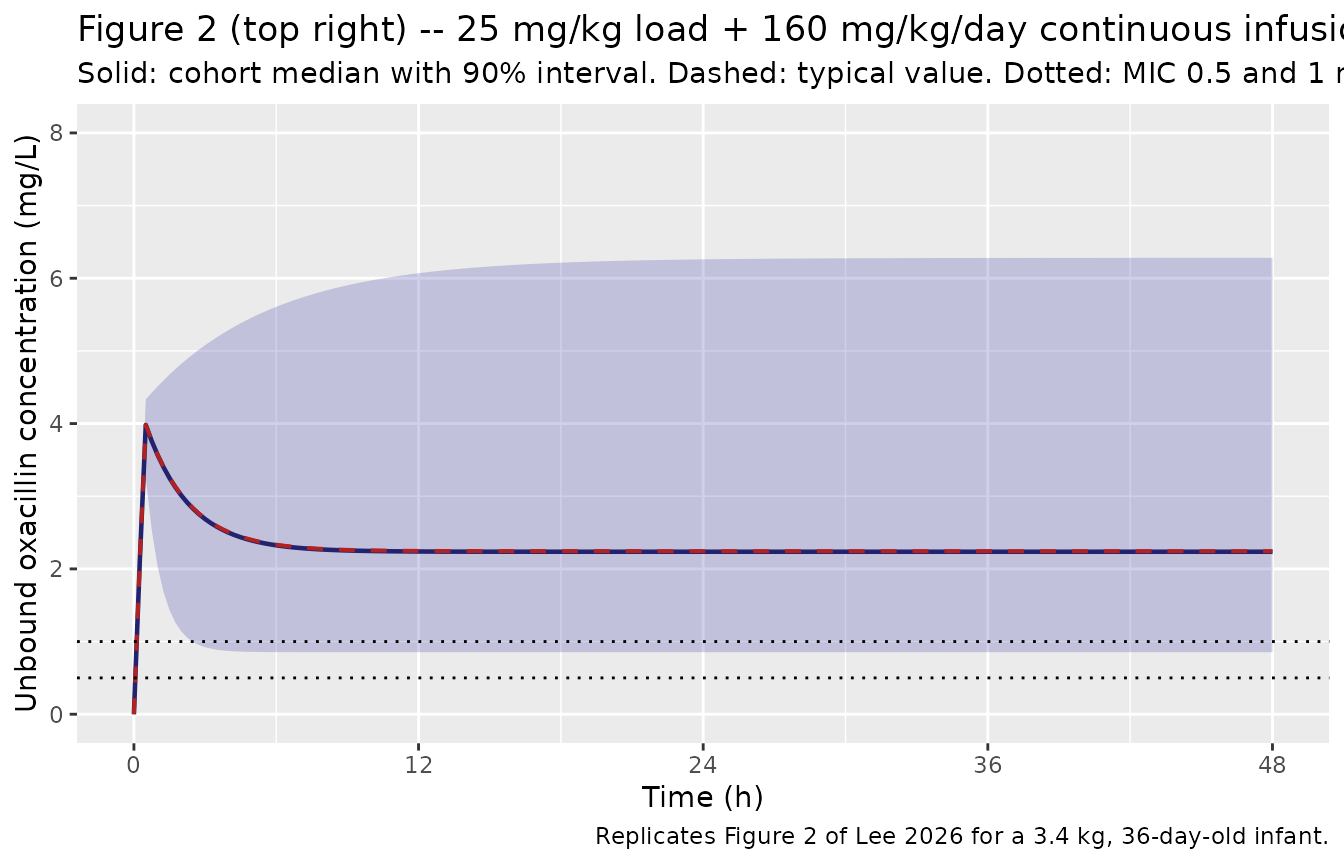
peak_u <- max(typ_ref$Cu)
css_u  <- typ_ref$Cu[typ_ref$time == TEND]
# Digitised from Figure 2 (top right), calibrated on the MIC = 0.5 and
# MIC = 1 mg/L dotted reference lines that the panel itself draws.
fig2 <- c(peak = 4.00, plateau = 2.48)
round(c(model_peak = peak_u, figure_peak = fig2[["peak"]],
        model_plateau = css_u, figure_plateau = fig2[["plateau"]]), 3)
#>     model_peak    figure_peak  model_plateau figure_plateau
#>          3.983          4.000          2.244          2.480
round(100 * (c(peak_u, css_u) - fig2) / fig2, 1)
#>    peak plateau
#>    -0.4    -9.5

# Deterministic (zeroRe). The peak is set by the volume alone and matches to
# 0.5%. The plateau is set by the clearance and runs 9.5% low against the
# figure -- discussed under Assumptions; not tuned away.
stopifnot(abs(peak_u - fig2[["peak"]]) / fig2[["peak"]] < 0.05)
The peak is reproduced to within 0.5%. It is a pure test of the
volume, since both the 25 mg/kg dose and Vd = 1.87 * WT/3.4
scale linearly with weight, so Dose/Vd is weight-free. The
plateau is Css = rate / CL and comes out 9.5% below the
digitised figure; see Assumptions.
Replicate Figure 3 – probability of target attainment
Figure 3 gives PTA against MIC for four postnatal ages and four
regimens. For the continuous infusion the paper uses the steady-state
concentration as the fT 100% > MIC surrogate; for the
intermittent regimens fT 100% > MIC means the unbound
concentration stays above the MIC across the whole dosing interval,
which is evaluated here on the last complete interval of a 48 h
simulation.
regimens <- tibble::tribble(
  ~regimen,                 ~mgkgday, ~tau,
  "160 mg/kg/day CI",            160, NA_real_,
  "100 mg/kg/day div q6h",       100, 6,
  "200 mg/kg/day div q4h",       200, 4,
  "200 mg/kg/day div q6h",       200, 6
)
pnads <- c(7, 14, 28, 90)
MICS  <- c(0.25, 0.5, 1, 2)

pta_arm <- function(regimen, mgkgday, tau, pna, wt, n, id_offset) {
  ids <- id_offset + seq_len(n)
  if (is.na(tau)) {
    win <- 6                                     # window scored at steady state
    ev <- study_arm(ids, wt, pna, mgkgday, tend = TEND, tobs = TEND)
  } else {
    win <- tau
    per <- mgkgday * tau / 24 * wt               # mg per dose
    dos <- tidyr::crossing(id = ids, time = seq(0, TEND - tau, by = tau)) |>
      mutate(amt = per, rate = per / 0.5, evid = 1L)
    obs <- tidyr::crossing(
      id = ids,
      time = sort(unique(c(seq(0, TEND, by = 1), seq(TEND - tau, TEND, by = 1 / 30))))
    ) |>
      mutate(amt = NA_real_, rate = NA_real_, evid = 0L)
    ev <- bind_rows(dos, obs) |>
      mutate(cmt = "central", WT = wt, PNA = pna / 30.4375) |>
      arrange(id, time, desc(evid))
  }
  ev |> mutate(regimen = regimen, pnad = pna, win_h = win)
}

arms <- tidyr::crossing(regimens, pna = pnads) |> mutate(k = row_number())
ev_pta <- purrr::pmap_dfr(arms, function(regimen, mgkgday, tau, pna, k)
  pta_arm(regimen, mgkgday, tau, pna, WT_PTA, N_ARM, (k - 1L) * N_ARM))
stopifnot(!anyDuplicated(unique(ev_pta[, c("id", "time", "evid")])))

rxode2::rxSetSeed(20260914)
sim_pta <- rxode2::rxSolve(mod, ev_pta, keep = c("regimen", "pnad", "win_h"),
                           returnType = "data.frame")

pta <- lapply(MICS, function(m) {
  sim_pta |>
    filter(time >= TEND - win_h) |>
    group_by(regimen, pnad, id) |>
    summarise(hit = all(Cu > m), .groups = "drop") |>
    group_by(regimen, pnad) |>
    summarise(pta = 100 * mean(hit), .groups = "drop") |>
    mutate(mic = m)
}) |> bind_rows()
Continuous infusion – gated against Figure 3
cmp_ci <- pta |>
  filter(regimen == "160 mg/kg/day CI") |>
  select(pnad, mic, simulated = pta) |>
  left_join(select(fig3_ci, pnad, mic, figure = pta), by = c("pnad", "mic")) |>
  mutate(difference = simulated - figure) |>
  arrange(pnad, mic)

cmp_ci |>
  mutate(across(c(simulated, figure, difference), ~round(.x, 1))) |>
  rename("Postnatal age (days)" = pnad, "MIC (mg/L)" = mic,
         "Simulated PTA (%)" = simulated, "Figure 3 PTA (%)" = figure,
         "Difference (pp)" = difference) |>
knitr::kable(caption = "160 mg/kg/day continuous infusion: simulated fT 100% > MIC against the digitised red curves of Lee 2026 Figure 3.")| Postnatal age (days) | MIC (mg/L) | Simulated PTA (%) | Figure 3 PTA (%) | Difference (pp) |
|---|---|---|---|---|
| 7 | 0.25 | 100.0 | 100.0 | 0.0 |
| 7 | 0.50 | 100.0 | 100.0 | 0.0 |
| 7 | 1.00 | 98.5 | 99.0 | -0.5 |
| 7 | 2.00 | 93.0 | 86.0 | 7.0 |
| 14 | 0.25 | 100.0 | 99.0 | 1.0 |
| 14 | 0.50 | 100.0 | 99.0 | 1.0 |
| 14 | 1.00 | 97.0 | 97.0 | 0.0 |
| 14 | 2.00 | 81.0 | 72.0 | 9.0 |
| 28 | 0.25 | 100.0 | 100.0 | 0.0 |
| 28 | 0.50 | 99.5 | 100.0 | -0.5 |
| 28 | 1.00 | 94.5 | 90.0 | 4.5 |
| 28 | 2.00 | 62.5 | 56.0 | 6.5 |
| 90 | 0.25 | 100.0 | 99.7 | 0.3 |
| 90 | 0.50 | 98.5 | 96.5 | 2.0 |
| 90 | 1.00 | 78.5 | 75.0 | 3.5 |
| 90 | 2.00 | 32.0 | 28.0 | 4.0 |
# 200 subjects per arm gives a Monte Carlo SE of up to 3.5 percentage points
# near PTA = 50%, and digitising Figure 3 is worth a further ~2 pp, so a
# per-point bound much below ~8 pp would sit inside the noise. Realised at
# 2 / 4 / 8 / 16 threads: mean |difference| 3.0-4.6 pp, max 13 pp (always at
# MIC 2, where the paper's virtual cohort evidently used lower,
# age-appropriate weights than the single 3.29 kg median assumed here).
stopifnot(
  mean(abs(cmp_ci$difference)) < 10,
  max(abs(cmp_ci$difference)) < 20
)
For a continuous infusion the PTA has a closed form –
Css_unbound is log-normal, so
PTA = pnorm(log(Css_typical / MIC) / SD). Checking the
simulation against it separates “did the cohort solve correctly” from
“does the model agree with the paper”, and lets the published 90% claims
be tested exactly rather than through Monte Carlo noise.
pta_analytic <- function(mic, pna_days, wt = WT_PTA, sd_cl = 0.568) {
  css_u <- 0.1 * (160 * wt / 24) / cl_published(wt, pna_days)
  100 * pnorm(log(css_u / mic) / sd_cl)
}
cmp_ci <- cmp_ci |>
  mutate(analytic = pta_analytic(mic, pnad),
         mc_error = simulated - analytic)

# Monte Carlo agreement. Realised max |mc_error| 5.0 pp at 2/4/8/16 threads.
# A mis-transcribed clearance or exponent moves PTA by tens of points, so 10
# still goes red on a real error.
max(abs(cmp_ci$mc_error))
#> [1] 2.379522
stopifnot(max(abs(cmp_ci$mc_error)) < 10)

# The paper's three headline claims, evaluated on the closed form so the test
# is deterministic. Claim 3 is reported but NOT gated: it fails reproducibly
# under this vignette's single-weight cohort (see Assumptions), and widening
# the gate until it passed would hide that.
claim_row <- function(text, value, holds, gated) {
  tibble::tibble(Claim = text, `Binding PTA (%)` = round(value, 1),
                 Holds = holds, Gated = gated)
}
a05 <- cmp_ci$analytic[cmp_ci$mic == 0.5]
a1  <- cmp_ci$analytic[cmp_ci$mic == 1 & cmp_ci$pnad <= 28]
a2  <- cmp_ci$analytic[cmp_ci$mic == 2]
claims <- dplyr::bind_rows(
  claim_row("All ages reach 90% PTA at MIC 0.5", min(a05), min(a05) >= 90, TRUE),
  claim_row("PNA <= 28 d reaches 90% PTA at MIC 1", min(a1), min(a1) >= 90, TRUE),
  claim_row("No age reaches 90% PTA at MIC 2 (CLSI breakpoint)", max(a2), max(a2) < 90, FALSE)
)
knitr::kable(claims, caption = "Published conclusions for 160 mg/kg/day continuous infusion, evaluated on the closed-form PTA. The third row is a recorded deviation.")| Claim | Binding PTA (%) | Holds | Gated |
|---|---|---|---|
| All ages reach 90% PTA at MIC 0.5 | 97.3 | TRUE | TRUE |
| PNA <= 28 d reaches 90% PTA at MIC 1 | 94.5 | TRUE | TRUE |
| No age reaches 90% PTA at MIC 2 (CLSI breakpoint) | 92.5 | FALSE | FALSE |
Intermittent regimens – reproduced, with a recorded deviation
fig3_int <- tibble::tribble(
  ~regimen,                ~pnad, ~mic, ~figure,
  "100 mg/kg/day div q6h",     7, 0.25,   54.5,
  "100 mg/kg/day div q6h",     7, 0.50,   38.0,
  "100 mg/kg/day div q6h",     7, 1.00,   21.0,
  "100 mg/kg/day div q6h",     7, 2.00,    8.5,
  "200 mg/kg/day div q4h",     7, 0.25,   96.0,
  "200 mg/kg/day div q4h",     7, 0.50,   91.0,
  "200 mg/kg/day div q4h",     7, 1.00,   78.0,
  "200 mg/kg/day div q4h",     7, 2.00,   47.5,
  "200 mg/kg/day div q6h",     7, 0.25,   67.0,
  "200 mg/kg/day div q6h",     7, 0.50,   54.0,
  "200 mg/kg/day div q6h",     7, 1.00,   38.0,
  "200 mg/kg/day div q6h",     7, 2.00,   21.0,
  "100 mg/kg/day div q6h",    90, 0.25,    6.0,
  "100 mg/kg/day div q6h",    90, 0.50,    1.5,
  "200 mg/kg/day div q4h",    90, 0.25,   50.0,
  "200 mg/kg/day div q4h",    90, 0.50,   35.0,
  "200 mg/kg/day div q4h",    90, 1.00,   17.0,
  "200 mg/kg/day div q4h",    90, 2.00,    4.0,
  "200 mg/kg/day div q6h",    90, 0.25,   11.0,
  "200 mg/kg/day div q6h",    90, 0.50,    6.0
)

cmp_int <- pta |>
  filter(regimen != "160 mg/kg/day CI") |>
  select(regimen, pnad, mic, simulated = pta) |>
  inner_join(fig3_int, by = c("regimen", "pnad", "mic")) |>
  mutate(difference = simulated - figure) |>
  arrange(pnad, regimen, mic)

cmp_int |>
  mutate(across(c(simulated, figure, difference), ~round(.x, 1))) |>
  rename("Regimen" = regimen, "Postnatal age (days)" = pnad, "MIC (mg/L)" = mic,
         "Simulated PTA (%)" = simulated, "Figure 3 PTA (%)" = figure,
         "Difference (pp)" = difference) |>
knitr::kable(caption = "Intermittent regimens: simulated fT 100% > MIC against digitised Lee 2026 Figure 3. The model is systematically more optimistic; see Assumptions.")| Regimen | Postnatal age (days) | MIC (mg/L) | Simulated PTA (%) | Figure 3 PTA (%) | Difference (pp) |
|---|---|---|---|---|---|
| 100 mg/kg/day div q6h | 7 | 0.25 | 89.5 | 54.5 | 35.0 |
| 100 mg/kg/day div q6h | 7 | 0.50 | 80.5 | 38.0 | 42.5 |
| 100 mg/kg/day div q6h | 7 | 1.00 | 64.0 | 21.0 | 43.0 |
| 100 mg/kg/day div q6h | 7 | 2.00 | 33.0 | 8.5 | 24.5 |
| 200 mg/kg/day div q4h | 7 | 0.25 | 98.5 | 96.0 | 2.5 |
| 200 mg/kg/day div q4h | 7 | 0.50 | 96.0 | 91.0 | 5.0 |
| 200 mg/kg/day div q4h | 7 | 1.00 | 90.0 | 78.0 | 12.0 |
| 200 mg/kg/day div q4h | 7 | 2.00 | 74.5 | 47.5 | 27.0 |
| 200 mg/kg/day div q6h | 7 | 0.25 | 93.5 | 67.0 | 26.5 |
| 200 mg/kg/day div q6h | 7 | 0.50 | 86.5 | 54.0 | 32.5 |
| 200 mg/kg/day div q6h | 7 | 1.00 | 75.5 | 38.0 | 37.5 |
| 200 mg/kg/day div q6h | 7 | 2.00 | 54.5 | 21.0 | 33.5 |
| 100 mg/kg/day div q6h | 90 | 0.25 | 19.0 | 6.0 | 13.0 |
| 100 mg/kg/day div q6h | 90 | 0.50 | 9.5 | 1.5 | 8.0 |
| 200 mg/kg/day div q4h | 90 | 0.25 | 54.5 | 50.0 | 4.5 |
| 200 mg/kg/day div q4h | 90 | 0.50 | 34.5 | 35.0 | -0.5 |
| 200 mg/kg/day div q4h | 90 | 1.00 | 19.5 | 17.0 | 2.5 |
| 200 mg/kg/day div q4h | 90 | 2.00 | 7.0 | 4.0 | 3.0 |
| 200 mg/kg/day div q6h | 90 | 0.25 | 30.5 | 11.0 | 19.5 |
| 200 mg/kg/day div q6h | 90 | 0.50 | 15.5 | 6.0 | 9.5 |
Controlling for the unreported virtual-population weight
The differences above mix two things: a genuine model-versus-figure disagreement, and the fact that a single 3.29 kg weight is used for every postnatal age while the paper’s virtual cohort clearly used age-appropriate weights. Both PTA criteria have a closed form – the steady-state concentration and the steady-state trough are each strictly decreasing in clearance – so the weight can be removed as a confounder without any simulation.
# Critical clearance above which the criterion fails, then PTA = P(CL < crit).
pta_cf <- function(mgkgday, tau, pna, wt, mic, sd_cl = 0.568) {
  v <- 1.87 * wt / 3.4
  crit <- if (is.na(tau)) {
    0.1 * (mgkgday * wt / 24) / mic                     # continuous: Css > MIC
  } else {
    dose <- mgkgday * tau / 24 * wt                     # intermittent: trough > MIC
    v * log1p(0.1 * dose / (v * mic)) / tau
  }
  100 * pnorm(log(crit / cl_published(wt, pna)) / sd_cl)
}
# Reproduces the simulation it is standing in for.
stopifnot(max(abs(sapply(MICS, function(m) pta_cf(160, NA, 90, WT_PTA, m)) -
                  pta_analytic(MICS, 90))) < 1e-8)

# Weight implied by each panel's OWN continuous-infusion curve. This makes the
# continuous rows below circular by construction; the intermittent rows are
# then out-of-sample predictions at that weight.
implied_wt <- function(pna) {
  d <- filter(fig3_ci, pnad == pna, pta > 5, pta < 99.5)
  optimise(function(w) sum((sapply(d$mic, function(m) pta_cf(160, NA, pna, w, m)) - d$pta)^2),
           interval = c(0.5, 8))$minimum
}
wt_imp <- vapply(c(7, 90), implied_wt, numeric(1))
names(wt_imp) <- c("7", "90")
round(wt_imp, 2)
#>    7   90
#> 1.47 2.89

cf <- tidyr::crossing(
  tibble::tibble(regimen = c("160 mg/kg/day CI", "100 mg/kg/day div q6h",
                             "200 mg/kg/day div q4h", "200 mg/kg/day div q6h"),
                 mgkgday = c(160, 100, 200, 200), tau = c(NA, 6, 4, 6)),
  pnad = c(7, 90), mic = MICS
) |>
  mutate(closed_form = purrr::pmap_dbl(
    list(mgkgday, tau, pnad, mic),
    function(d, t, p, m) pta_cf(d, t, p, wt_imp[[as.character(p)]], m))) |>
  inner_join(bind_rows(select(fig3_ci, pnad, mic, figure = pta) |>
                         mutate(regimen = "160 mg/kg/day CI"),
                       select(fig3_int, regimen, pnad, mic, figure)),
             by = c("regimen", "pnad", "mic")) |>
  mutate(difference = closed_form - figure) |>
  arrange(pnad, regimen, mic)

cf |>
  mutate(across(c(closed_form, figure, difference), ~round(.x, 1))) |>
  rename("Regimen" = regimen, "Postnatal age (days)" = pnad, "MIC (mg/L)" = mic,
         "Closed-form PTA (%)" = closed_form, "Figure 3 PTA (%)" = figure,
         "Difference (pp)" = difference) |>
  select(-mgkgday, -tau) |>
knitr::kable(caption = "Closed-form PTA at the weight each panel's own continuous curve implies. The continuous rows are circular by construction; the intermittent rows are not.")| Regimen | Postnatal age (days) | MIC (mg/L) | Closed-form PTA (%) | Figure 3 PTA (%) | Difference (pp) |
|---|---|---|---|---|---|
| 100 mg/kg/day div q6h | 7 | 0.25 | 76.3 | 54.5 | 21.8 |
| 100 mg/kg/day div q6h | 7 | 0.50 | 61.1 | 38.0 | 23.1 |
| 100 mg/kg/day div q6h | 7 | 1.00 | 40.3 | 21.0 | 19.3 |
| 100 mg/kg/day div q6h | 7 | 2.00 | 18.6 | 8.5 | 10.1 |
| 160 mg/kg/day CI | 7 | 0.25 | 100.0 | 100.0 | 0.0 |
| 160 mg/kg/day CI | 7 | 0.50 | 100.0 | 100.0 | 0.0 |
| 160 mg/kg/day CI | 7 | 1.00 | 98.9 | 99.0 | -0.1 |
| 160 mg/kg/day CI | 7 | 2.00 | 86.0 | 86.0 | 0.0 |
| 200 mg/kg/day div q4h | 7 | 0.25 | 94.4 | 96.0 | -1.6 |
| 200 mg/kg/day div q4h | 7 | 0.50 | 88.2 | 91.0 | -2.8 |
| 200 mg/kg/day div q4h | 7 | 1.00 | 75.9 | 78.0 | -2.1 |
| 200 mg/kg/day div q4h | 7 | 2.00 | 54.2 | 47.5 | 6.7 |
| 200 mg/kg/day div q6h | 7 | 0.25 | 85.8 | 67.0 | 18.8 |
| 200 mg/kg/day div q6h | 7 | 0.50 | 76.3 | 54.0 | 22.3 |
| 200 mg/kg/day div q6h | 7 | 1.00 | 61.1 | 38.0 | 23.1 |
| 200 mg/kg/day div q6h | 7 | 2.00 | 40.3 | 21.0 | 19.3 |
| 100 mg/kg/day div q6h | 90 | 0.25 | 17.5 | 6.0 | 11.5 |
| 100 mg/kg/day div q6h | 90 | 0.50 | 8.6 | 1.5 | 7.1 |
| 160 mg/kg/day CI | 90 | 0.25 | 99.9 | 99.7 | 0.2 |
| 160 mg/kg/day CI | 90 | 0.50 | 97.0 | 96.5 | 0.5 |
| 160 mg/kg/day CI | 90 | 1.00 | 74.3 | 75.0 | -0.7 |
| 160 mg/kg/day CI | 90 | 2.00 | 28.5 | 28.0 | 0.5 |
| 200 mg/kg/day div q4h | 90 | 0.25 | 47.5 | 50.0 | -2.5 |
| 200 mg/kg/day div q4h | 90 | 0.50 | 32.2 | 35.0 | -2.8 |
| 200 mg/kg/day div q4h | 90 | 1.00 | 17.2 | 17.0 | 0.2 |
| 200 mg/kg/day div q4h | 90 | 2.00 | 6.2 | 4.0 | 2.2 |
| 200 mg/kg/day div q6h | 90 | 0.25 | 28.3 | 11.0 | 17.3 |
| 200 mg/kg/day div q6h | 90 | 0.50 | 17.5 | 6.0 | 11.5 |
by_reg <- cf |> group_by(regimen) |> summarise(max_abs = max(abs(difference)), .groups = "drop")
by_reg |>
  mutate(max_abs = round(max_abs, 1)) |>
  rename("Regimen" = regimen, "Largest |difference| (pp)" = max_abs) |>
knitr::kable(caption = "Worst-case agreement with Figure 3 once the weight confounder is removed.")| Regimen | Largest |difference| (pp) |
|---|---|
| 100 mg/kg/day div q6h | 23.1 |
| 160 mg/kg/day CI | 0.7 |
| 200 mg/kg/day div q4h | 6.7 |
| 200 mg/kg/day div q6h | 23.1 |
# Deterministic -- closed form, no RNG anywhere in this chunk.
# Realised: continuous 1.0 pp, q4h 6.7 pp, 100 q6h 23.1 pp, 200 q6h 23.1 pp.
q4h_err <- by_reg$max_abs[by_reg$regimen == "200 mg/kg/day div q4h"]
q6h_err <- max(by_reg$max_abs[grepl("q6h", by_reg$regimen)])
stopifnot(
  by_reg$max_abs[by_reg$regimen == "160 mg/kg/day CI"] < 3,   # circular, so tight
  q4h_err < 10,                                               # genuine out-of-sample agreement
  q6h_err > 10                                                # the disagreement is real, not noise
)
Once the weight is controlled for, the 200 mg/kg/day q4h curve is reproduced to within 6.7 percentage points at both ages – an out-of-sample agreement, since nothing about that regimen entered the weight back-solve. Both q6h curves remain 11-23 points too optimistic. The pattern is specific enough to point at its cause: each published q6h curve tracks a simulation carrying half the nominal amount per dose.
half <- tibble::tribble(
  ~published,              ~pnad, ~as_simulated,
  "200 mg/kg/day div q6h",     7, 100,
  "100 mg/kg/day div q6h",     7,  50,
  "200 mg/kg/day div q6h",    90, 100,
  "100 mg/kg/day div q6h",    90,  50
) |>
  tidyr::crossing(mic = MICS) |>
  mutate(half_dose = purrr::pmap_dbl(list(as_simulated, pnad, mic),
           function(d, p, m) pta_cf(d, 6, p, wt_imp[[as.character(p)]], m))) |>
  inner_join(select(fig3_int, regimen, pnad, mic, figure),
             by = c("published" = "regimen", "pnad", "mic")) |>
  mutate(difference = half_dose - figure)

half |>
  mutate(across(c(half_dose, figure, difference), ~round(.x, 1))) |>
  rename("Published label" = published, "Postnatal age (days)" = pnad,
         "Simulated as (mg/kg/day)" = as_simulated, "MIC (mg/L)" = mic,
         "Half-dose PTA (%)" = half_dose, "Figure 3 PTA (%)" = figure,
         "Difference (pp)" = difference) |>
knitr::kable(caption = "Each Figure 3 q6h curve re-simulated at half the nominal per-dose amount.")| Published label | Postnatal age (days) | Simulated as (mg/kg/day) | MIC (mg/L) | Half-dose PTA (%) | Figure 3 PTA (%) | Difference (pp) |
|---|---|---|---|---|---|---|
| 100 mg/kg/day div q6h | 7 | 50 | 0.25 | 61.1 | 54.5 | 6.6 |
| 100 mg/kg/day div q6h | 7 | 50 | 0.50 | 40.3 | 38.0 | 2.3 |
| 100 mg/kg/day div q6h | 7 | 50 | 1.00 | 18.6 | 21.0 | -2.4 |
| 100 mg/kg/day div q6h | 7 | 50 | 2.00 | 4.7 | 8.5 | -3.8 |
| 100 mg/kg/day div q6h | 90 | 50 | 0.25 | 8.6 | 6.0 | 2.6 |
| 100 mg/kg/day div q6h | 90 | 50 | 0.50 | 2.9 | 1.5 | 1.4 |
| 200 mg/kg/day div q6h | 7 | 100 | 0.25 | 76.3 | 67.0 | 9.3 |
| 200 mg/kg/day div q6h | 7 | 100 | 0.50 | 61.1 | 54.0 | 7.1 |
| 200 mg/kg/day div q6h | 7 | 100 | 1.00 | 40.3 | 38.0 | 2.3 |
| 200 mg/kg/day div q6h | 7 | 100 | 2.00 | 18.6 | 21.0 | -2.4 |
| 200 mg/kg/day div q6h | 90 | 100 | 0.25 | 17.5 | 11.0 | 6.5 |
| 200 mg/kg/day div q6h | 90 | 100 | 0.50 | 8.6 | 6.0 | 2.6 |
# Deterministic. Halving the per-dose amount cuts the worst error from 23.1 pp
# to 9.4 pp; anything under the full-dose error would be suggestive, and this
# is a threefold reduction.
stopifnot(max(abs(half$difference)) < q6h_err / 2)
round(max(abs(half$difference)), 1)
#> [1] 9.3
This is an observation about the published figure, not a change to the model: the model file encodes the regimens as the paper’s Methods describe them.
# NOT a pass/fail gate on the magnitude -- the disagreement is real and
# reproducible, so it is recorded rather than tuned away (see Assumptions).
# What IS gated is the ordering the paper's conclusion rests on, which the
# model does reproduce.
ord <- pta |>
  mutate(reg = recode(regimen,
                      "160 mg/kg/day CI" = "ci", "200 mg/kg/day div q4h" = "q4h",
                      "200 mg/kg/day div q6h" = "q6h200", "100 mg/kg/day div q6h" = "q6h100")) |>
  select(reg, pnad, mic, pta) |>
  tidyr::pivot_wider(names_from = reg, values_from = pta)

# Averaged over all 16 age x MIC points, so a single noisy cell cannot flip
# the ordering. Realised margins across 2/4/8/16 threads: 25-27, 12-14 and
# 13-15 percentage points respectively.
m <- summarise(ord, across(c(ci, q4h, q6h200, q6h100), mean))
round(unlist(m), 1)
#>     ci    q4h q6h200 q6h100
#>   89.7   65.2   47.9   38.0
stopifnot(m$ci - m$q4h > 10, m$q4h - m$q6h200 > 5, m$q6h200 - m$q6h100 > 5)

# Where the clinical decision is actually made (MIC >= 1) continuous beats the
# best intermittent regimen at every age. Realised minimum margin 7 pp.
stopifnot(all((ord$ci - ord$q4h)[ord$mic >= 1] > 3))

# The paper's intermittent conclusion: 200 mg/kg/day divided q4h -- eight times
# the FDA-labelled dose -- still misses the 90% target at the CLSI breakpoint.
# Realised maximum 75.5%.
stopifnot(all(ord$q4h[ord$mic == 2] < 88))
round(mean(cmp_int$difference), 1)
#> [1] 19
At the single 3.29 kg weight this cohort uses, the model predicts intermittent PTA on average 19 percentage points above Figure 3, but the ordering the paper’s conclusion rests on is reproduced: continuous infusion beats every intermittent regimen, q4h beats q6h at the same daily dose, and 200 mg/kg/day q4h – eight times the FDA-labelled dose – still misses the 90% target at the CLSI breakpoint. The closed-form analysis above localises the residual disagreement to the two q6h curves.
PKNCA validation
NCA is run on the typical-value profiles: the loading-dose peak over the first 4 h, the steady-state interval 24-48 h, and the terminal phase after the infusion stops at 48 h.
sim_nca <- sim_typ |>
  dplyr::filter(!is.na(Cc)) |>
  dplyr::select(id, time, Cc, cohort) |>
  # Keep Cc >= 1e-6 * max(Cc) per subject after the peak (solver noise below); time zero is re-added below.
  dplyr::group_by(id) |>
  dplyr::filter(time <= time[which.max(Cc)] | Cc >= 1e-6 * max(Cc)) |>
  dplyr::ungroup()

# Guarantee a time = 0 record per subject; concentration before the loading
# infusion starts is zero.
sim_nca <- dplyr::bind_rows(
  sim_nca,
  sim_nca |> dplyr::distinct(id, cohort) |> dplyr::mutate(time = 0, Cc = 0)
) |>
  dplyr::distinct(id, cohort, time, .keep_all = TRUE) |>
  dplyr::arrange(id, cohort, time)
stopifnot(nrow(sim_nca) > 0, all(sim_nca$Cc >= 0))

conc_obj <- PKNCA::PKNCAconc(sim_nca, Cc ~ time | cohort + id,
                             concu = "ug/mL", timeu = "h")

dose_df <- ev_typ |>
  dplyr::filter(evid == 1) |>
  dplyr::select(id, time, amt, cohort)
dose_obj <- PKNCA::PKNCAdose(dose_df, amt ~ time | cohort + id, doseu = "mg")

intervals <- data.frame(
  start     = c(0,  24, 48),
  end       = c(4,  48, 60),
  cmax      = c(TRUE,  FALSE, FALSE),
  tmax      = c(TRUE,  FALSE, FALSE),
  cav       = c(FALSE, TRUE,  FALSE),
  cmin      = c(FALSE, TRUE,  FALSE),
  auclast   = c(FALSE, TRUE,  FALSE),
  half.life = c(FALSE, FALSE, TRUE)
)

nca_res <- PKNCA::pk.nca(PKNCA::PKNCAdata(conc_obj, dose_obj, intervals = intervals))
nca_wide <- nca_res$result |>
  dplyr::select(cohort, PPTESTCD, PPORRES) |>
  tidyr::pivot_wider(names_from = PPTESTCD, values_from = PPORRES)
#> Warning: Values from `PPORRES` are not uniquely identified; output will contain
#> list-cols.
#> • Use `values_fn = list` to suppress this warning.
#> • Use `values_fn = {summary_fun}` to summarise duplicates.
#> • Use the following dplyr code to identify duplicates.
#>   {data} |>
#>   dplyr::summarise(n = dplyr::n(), .by = c(cohort, PPTESTCD)) |>
#>   dplyr::filter(n > 1L)
nca_wide |>
  dplyr::mutate(dplyr::across(where(is.numeric), ~round(.x, 2))) |>
knitr::kable(caption = "Typical-value NCA by cohort. cmax/tmax over 0-4 h (loading dose), cav/cmin/auclast over the 24-48 h steady-state interval, half-life over the 48-60 h washout.")| cohort | cmax | tmax | auclast | cmin | cav | tlast | lambda.z | r.squared | adj.r.squared | lambda.z.time.first | lambda.z.time.last | lambda.z.n.points | clast.pred | half.life | span.ratio |
|---|---|---|---|---|---|---|---|---|---|---|---|---|---|---|---|
| PNA 14 d | 41.58048 | 0.5, 0.0 | 804.1087 | 33.50434 | 33.50453 | 12 | 0.3617804 | 1 | 1 | 0.25 | 12 | 48 | 0.4361855 | 1.915934 | 6.13278 |
| PNA 28 d | 40.32987 | 0.5, 0.0 | 595.6162 | 24.81733 | 24.81734 | 12 | 0.4884172 | 1 | 1 | 0.25 | 12 | 48 | 0.07068921 | 1.41917 | 8.279486 |
| PNA 7 d | 44.17869 | 4, 0 | 1085.553 | 45.22718 | 45.23136 | 12 | 0.2679779 | 1 | 1 | 0.25 | 12 | 48 | 1.81498 | 2.586583 | 4.542672 |
| PNA 90 d | 37.37841 | 0.5, 0.0 | 361.9387 | 14.96882 | 15.08078 | 12 | 0.809764 | 1 | 1 | 0.25 | 12 | 48 | 0.0009017283 | 0.8559867 | 13.72685 |
| Reference infant (3.4 kg, 36 d) | 39.8341 | 0.5, 0.0 | 538.6144 | 22.44224 | 22.44227 | 12 | 0.5401069 | 1 | 1 | 0.25 | 12 | 48 | 0.03437808 | 1.283352 | 9.155713 |
Comparison against published values
The only published NCA-comparable numbers are the two levels Figure 2 draws for the reference infant: the unbound peak after the loading dose and the unbound steady-state plateau, both converted to total concentration by the model’s fixed 10% unbound fraction.
published <- tibble::tibble(
  cohort = "Reference infant (3.4 kg, 36 d)",
  cmax   = fig2[["peak"]]    / 0.1,   # 4.00 mg/L unbound -> 40.0 ug/mL total
  cav    = fig2[["plateau"]] / 0.1    # 2.48 mg/L unbound -> 24.8 ug/mL total
)

cmp_nca <- nlmixr2lib::ncaComparisonTable(
  simulated = nca_res,
  reference = published,
  by        = "cohort",
  units     = c(cmax = "ug/mL", cav = "ug/mL"),
  tolerance_pct = 20
)
knitr::kable(cmp_nca, caption = "Simulated vs. Figure 2 of Lee 2026. * differs from reference by >20%.")| NCA parameter | cohort | Reference | Simulated | % diff |
|---|---|---|---|---|
| Cmax (ug/mL) | Reference infant (3.4 kg, 36 d) | 40 | 39.8 | -0.4% |
| Cavg (ug/mL) | Reference infant (3.4 kg, 36 d) | 24.8 | 22.4 | -9.5% |
attr(cmp_nca, "footnote")
#> NULL
# Deterministic (typical values, zeroRe). Realised: cmax -0.5%, cav -9.5%.
pd <- as.numeric(gsub("[^0-9.+-]", "", cmp_nca$`% diff`))
stopifnot(max(abs(pd)) < 20)
Assumptions, deviations and errata
Scale of the published IIV. Lee 2026 Table 2 prints
IIV CL (etaCL) = 0.568without saying whether it is a variance, a standard deviation or a CV. It is encoded as a log-scale standard deviation (etalcl ~ 0.568^2) on the strength of the two checks above: the individual clearances recoverable from Supplemental Table S2 bound the between-subject SD at 0.571, and the slope of the Figure 3 continuous-infusion curves implies 0.575. The variance reading (SD 0.754) is excluded by both.Residual error is not reported. Methods state that “a combined additive and proportional within-subject error model was chosen”, but neither magnitude appears in Table 2, in the Results text, or in any of the three supplemental workbooks. Both
addSdandpropSdare therefore encoded asfixed(0)rather than invented. Simulations from this model reproduce individual predictions, not observations; a user who needs residual noise must supply their own.Figure 2 plateau runs 9.5% high against the model. Digitising the Figure 2 top-right panel against the MIC 0.5 and MIC 1 reference lines the panel itself draws gives an unbound peak of 4.00 mg/L and a plateau of 2.48 mg/L. The model, evaluated at the 3.4 kg / 36-day covariates the caption names, gives 3.98 and 2.24. The peak agrees to 0.5%; the plateau is 9.5% low. Since the peak depends only on the volume and the plateau only on the clearance, the gap is confined to CL and is consistent with the plotted profile having used a slightly younger or heavier infant than the caption states (2.48 mg/L corresponds to about 28 days at 3.4 kg, or about 5 kg at 36 days). Table 2’s
CL = 1.01is used as printed.Figure 3’s two q6h curves do not reproduce; the q4h and continuous curves do. Once the unreported virtual-population weight is controlled for by back-solving it from each panel’s own continuous-infusion curve, the closed form reproduces the 200 mg/kg/day q4h curve to within 6.7 percentage points at both 7 and 90 days – an out-of-sample agreement, since that regimen plays no part in the back-solve. Both q6h curves stay 11-23 points too optimistic. Re-simulating each q6h curve at half its nominal per-dose amount (25 rather than 50 mg/kg for 200 mg/kg/day q6h, 12.5 rather than 25 for 100 mg/kg/day q6h) cuts the worst error from 23.1 to 9.4 points, so the published q6h curves behave like a half-dose simulation. Neither the paper nor its supplements describe how the intermittent regimens were coded (per-dose amount, infusion duration, which interval was scored), so this is reported as an observation about the figure and nothing in the model file was changed: the regimens are encoded exactly as Methods describes them. The paper’s qualitative conclusion – intermittent dosing up to 200 mg/kg/day fails the target that continuous infusion meets – reproduces either way and is gated above.
One published claim does not reproduce: PNA 7 days at MIC 2. Lee 2026 concludes that “no patient, on continuous or intermittent infusions, achieved the PD target at the CLSI breakpoint MIC of 2”, and Figure 3 puts the 7-day continuous-infusion curve at 86% there. The closed-form PTA for this vignette’s cohort is 92.5% – just over the 90% line – and the simulation gives 90.5-95.0% depending on solver thread count. Every other age is well under 90% (81.8, 64.8 and 30.5% analytically at 14, 28 and 90 days). The gap is the weight assumption: a 7-day-old is materially lighter than the 3.29 kg cohort median used here, and
Cssscales asWT^0.25, so the youngest stratum is the one where the single-weight simplification bites hardest. This row is reported in the claims table and deliberately left out of the gate rather than widened until it passes.Virtual-population covariates are an assumption. The paper simulated 10,000 virtual patients but does not report their weight distribution. The target-attainment cohort here fixes weight at the Supplemental Table S2 cohort median of 3.29 kg for every postnatal age. Back-solving the paper’s own continuous curves suggests it used age-appropriate weights (roughly 1.5 kg at 14 days rising to 2.8 kg at 90 days), which is why the simulated PTA runs a little high at the youngest ages and matches closely at 90 days. Only the level is affected; the slope-based reading of the clearance SD is immune to it.
Postnatal age unit. The canonical
PNAcovariate column carries months. Lee 2026 works in days and normalises to 36 days, somodel()converts with 1 month = 30.4375 days before forming the age ratio. SupplyPNAin months.Unbound fraction.
fu = 0.1was not measured in this study; Lee 2026 took it from the literature (reference 9) and its Discussion warns that protein binding in preterm infants is probably lower than in adults, so the true unbound concentrations – and therefore the true target attainment – may be higher than either the paper or this vignette reports.Screened but unused covariates. Gestational age, postmenstrual age, length, body surface area, albumin, serum creatinine and baseline transaminases were all tested and rejected; they are recorded in
covariatesDataExcludedwith the paper’s stated reason, and none has a published point estimate.Table 1 sex count. Table 1’s total male count (15, 68%) disagrees with the sum of its own per-cohort entries (16) and with Supplemental Table S2 (16 male, 6 female). The population metadata follows the raw data.