Model and source
- Citation: Por ED, Akers KS, Chung KK, Livezey JR, Selig DJ. Population pharmacokinetic modeling and simulations of imipenem in burn patients with and without continuous venovenous hemofiltration in the military health system. J Clin Pharmacol. 2021;61(9):1182-1194. doi:10.1002/jcph.1865. This model is also catalogued (as study 12) by Zhang P, Zhao Y, Zhu J, Yang Y, Liang G, Wang X, Yu Z. Population pharmacokinetics of imipenem in different populations for individualized dosing: a systematic review. Front Pharmacol. 2025;16:1738055. doi:10.3389/fphar.2025.1738055.
- Description: Two-compartment IV population PK model for imipenem in 23 US adult burn patients with (n = 12) and without (n = 11) continuous venovenous haemofiltration (Por 2021). Body clearance has two branches: patients not on CVVH carry power effects of Cockcroft-Gault creatinine clearance and body weight, while patients on CVVH carry a 10% lower clearance (categorical CVVH effect) with a body-weight effect only, plus their individual measured haemofilter clearance supplied as a covariate. Both volumes carry an inverse power effect of serum albumin and the central volume also scales with body weight. The creatinine clearance and weight exponents, Q and the peripheral volume were fixed from the literature. Inter-individual variability is exponential on clearance and the central volume, and residual error is proportional.
- Article: https://doi.org/10.1002/jcph.1865 (open access, PMC8453752)
Por et al. fitted a two-compartment model to steady-state imipenem concentrations from 23 adults with severe burns at the US Army Institute of Surgical Research Burn Center, 12 of them on continuous venovenous haemofiltration (CVVH). The final model combines the study’s own estimates (clearance, central volume, the CVVH effect, the albumin effects and the random effects) with values fixed from the literature: the creatinine clearance and body weight exponents come from the Bhagunde 2019 imipenem/relebactam model, and Q and the peripheral volume come from earlier imipenem studies.
This model was first added to nlmixr2lib from the Zhang
2025 imipenem review (Zhang 2025 review
article). It has since been rewritten from the primary publication
and its supplement; the section “Changes from the review-transcribed
version” lists what that re-verification changed.
Population
Twenty-three patients were enrolled: 11 without CVVH (1 woman, 10 men) and 12 with CVVH (5 women, 7 men). One patient had no post-dose sample and was excluded, leaving 81 prefilter plasma concentrations from 22 patients (Por 2021 Methods, Data). Mean (SD) age was 51.09 (19.03) years without and 55 (19.99) years with CVVH; weight 105.06 (28.66) and 89.6 (22.38) kg; total burn surface area 40.18% (20.88) and 45.31% (22.66); albumin 2.6 (0.55) and 2.92 (0.91) g/dL; Cockcroft-Gault creatinine clearance 151.92 (51.07) and 113.02 (58.92) mL/min (Table 1). The covariate medians used as reference values were weight 99.5 kg (range 57.9-150.8), albumin 2.7 g/dL (1.5-3.5) and, in the no-CVVH group only, CrCl 145.83 mL/min (88.08-253.95). Mean CVVH clearance was 1.56 (0.7) L/h. Nearly all patients received 500 mg every 6 h infused over 30 min or 1 h.
str(rxode2::rxode(readModelDb("Por_2021_imipenem"))$population)
#> ℹ parameter labels from comments will be replaced by 'label()'
#> List of 13
#>  $ species         : chr "human"
#>  $ n_subjects      : int 22
#>  $ n_studies       : int 1
#>  $ age_mean        : chr "51.09 +/- 19.03 years without CVVH; 55 +/- 19.99 years with CVVH (mean +/- SD)"
#>  $ weight_mean     : chr "105.06 +/- 28.66 kg without CVVH; 89.6 +/- 22.38 kg with CVVH (mean +/- SD)"
#>  $ weight_range    : chr "57.9-150.8 kg (median 99.5 kg)"
#>  $ sex_female_pct  : num 26.1
#>  $ race_ethnicity  : NULL
#>  $ disease_state   : chr "Adult patients with severe burns (mean total burn surface area 40% without and 45% with CVVH) at the US Army In"| __truncated__
#>  $ dose_range      : chr "500 mg imipenem every 6 h infused over 30 min or 1 h in 21 patients; one patient 1000 mg every 6 h over 1 h and"| __truncated__
#>  $ regions         : chr "United States of America"
#>  $ n_concentrations: int 81
#>  $ notes           : chr "23 patients enrolled (11 without and 12 with CVVH; 1 woman and 10 men without, 5 women and 7 men with); one had"| __truncated__
Source trace
| Equation / parameter | Value | Source location |
|---|---|---|
lcl (CL, no CVVH, reference subject) |
15.31 L/h | Table 2; Equation 10 |
lvc (Vc) |
32.67 L | Table 2; Equation 12 |
lq (Q) |
11 L/h, fixed | Table 2, footnote a |
lvp (Vp) |
41.23 L, fixed | Table 2, footnote b; Equation 13 |
e_rrt_crrt_status_cl |
-0.1 | Table 2 ‘CVVH (categorical)’; Equation 7 form; 15.31 x 0.9 = 13.78 in Equation 11 |
e_crcl_cl |
0.46, fixed | Table 2, footnote c (Bhagunde 2019); Equation 10 |
e_wt_cl |
0.33, fixed | Table 2, footnote c; Equation 10 |
e_wt_cl_cvvh |
0.75, fixed | Table 2; Equation 11 |
e_wt_vc |
0.74, fixed | Table 2, footnote c; Equation 12 |
e_alb_vc |
-1.17 | Table 2; Equation 12 |
e_alb_vp |
-3.68 | Table 2; Equation 13 |
etalcl |
variance 0.093 | Table 2 ‘omega2 CL’ |
etalvc |
variance 0.13 | Table 2 ‘omega2 Vc’ |
propSd |
0.3 | Table 2 ‘Proportional error’ |
CVVH clearance QEFF added after the eta |
per patient | Equations 1-3 and 5; Table 1 |
| Reference values 99.5 kg, 2.7 g/dL, 145.83 mL/min | Results, Patient Demographics | |
| Two-compartment structure, proportional error | Results, Base Model; Table S1 run 21 |
Changes from the review-transcribed version
| Item | Review-transcribed version | Re-verified from Por 2021 |
|---|---|---|
| IIV on CL (variance) | log(1 + 0.305^2) = 0.0889 | 0.093 (Table 2 prints omega^2) |
| IIV on Vc (variance) | log(1 + 0.361^2) = 0.1225 | 0.13 (Table 2 prints omega^2) |
| CVVH clearance | constant 1.56 L/h | per-patient covariate QEFF (1.56 is the cohort mean) |
| CVVH intercept 13.78 L/h | separate parameter | 15.31 x (1 - 0.1), the categorical effect of Table 2 |
| Fixed parameters | not marked | Q, Vp and four covariate exponents in fixed() |
| Sex split | 17 women, 6 men | 6 women, 17 men (Table 1) |
The review printed the IIV of this study as 30.5% and 36.1%, which
are the square roots of the variances in Por 2021 Table 2. The
review-wide reading omega^2 = log(1 + CV^2) therefore
understated both variances by 4-6%.
Deterministic checks against Table 3
Table 3 of Por 2021 lists the final model’s predicted typical Vc, Vp and CL for three reference populations. The model reproduces all three rows. The renal-impairment row matches only when its weight and creatinine clearance are exchanged: the printed “weight, 58 kg; CrCl, 54.1 mL/min” gives CL 8.12 L/h and Vc 13.84 L, but weight 54.1 kg with CrCl 58 mL/min gives the printed 8.19 L/h and 13.14 L to the last digit. The table’s two labels are evidently transposed; both readings are shown below.
mod <- rxode2::rxode(readModelDb("Por_2021_imipenem"))
#> ℹ parameter labels from comments will be replaced by 'label()'
m0 <- rxode2::zeroRe(mod)

tab3 <- tibble::tribble(
  ~Population, ~ALB_gdL, ~WT, ~CRCL, ~Vc_pub, ~Vp_pub, ~CL_pub,
  "Healthy", 4, 76, 106, 16.89, 9.7, 12.1,
  "Renal impairment (as printed)", 4, 58, 54.1, 13.14, 9.7, 8.19,
  "Renal impairment (weight and CrCl exchanged)", 4, 54.1, 58, 13.14, 9.7, 8.19,
  "Burn", 3, 70.8, 126.3, 22.45, 27.98, 12.81
)

typical <- function(ALB_gdL, WT, CRCL) {
  ev <- data.frame(
    id = 1L, time = c(0, 0.5), evid = c(1L, 0L), amt = c(500, 0),
    cmt = "central", ALB = ALB_gdL * 10, WT = WT, CRCL = CRCL,
    RRT_CRRT_STATUS = 0, QEFF = 0
  )
  s <- rxode2::rxSolve(m0, ev, returnType = "data.frame")
  s[1, c("vc", "vp", "cl")]
}

tab3_sim <- dplyr::bind_rows(lapply(seq_len(nrow(tab3)), function(i) {
  typical(tab3$ALB_gdL[i], tab3$WT[i], tab3$CRCL[i])
}))
#> ℹ omega/sigma items treated as zero: 'etalcl', 'etalvc'
#> ℹ omega/sigma items treated as zero: 'etalcl', 'etalvc'
#> ℹ omega/sigma items treated as zero: 'etalcl', 'etalvc'
#> ℹ omega/sigma items treated as zero: 'etalcl', 'etalvc'
tab3_cmp <- dplyr::bind_cols(tab3, tab3_sim) |>
  dplyr::mutate(dplyr::across(c(vc, vp, cl), \(x) round(x, 2)))

tab3_cmp |>
  dplyr::select(
    Population,
    "Vc sim (L)" = vc, "Vc Table 3" = Vc_pub,
    "Vp sim (L)" = vp, "Vp Table 3" = Vp_pub,
    "CL sim (L/h)" = cl, "CL Table 3" = CL_pub
  ) |>
knitr::kable(caption = "Replicates Table 3 of Por 2021.")| Population | Vc sim (L) | Vc Table 3 | Vp sim (L) | Vp Table 3 | CL sim (L/h) | CL Table 3 |
|---|---|---|---|---|---|---|
| Healthy | 16.90 | 16.89 | 9.71 | 9.70 | 12.10 | 12.10 |
| Renal impairment (as printed) | 13.84 | 13.14 | 9.71 | 9.70 | 8.12 | 8.19 |
| Renal impairment (weight and CrCl exchanged) | 13.14 | 13.14 | 9.71 | 9.70 | 8.19 | 8.19 |
| Burn | 22.45 | 22.45 | 27.98 | 27.98 | 12.81 | 12.81 |
# Deterministic: every row except the as-printed renal row must agree to
# the table's rounding.
gate3 <- dplyr::filter(tab3_cmp, Population != "Renal impairment (as printed)")
stopifnot(
  nrow(gate3) == 3L,
  all(abs(gate3$vc / gate3$Vc_pub - 1) < 0.005),
  all(abs(gate3$vp / gate3$Vp_pub - 1) < 0.005),
  all(abs(gate3$cl / gate3$CL_pub - 1) < 0.005)
)
# The burn row also prints total volume Vc + Vp = 50.43 L.
stopifnot(abs(sum(tab3_cmp[tab3_cmp$Population == "Burn", c("vc", "vp")]) - 50.43) < 0.02)
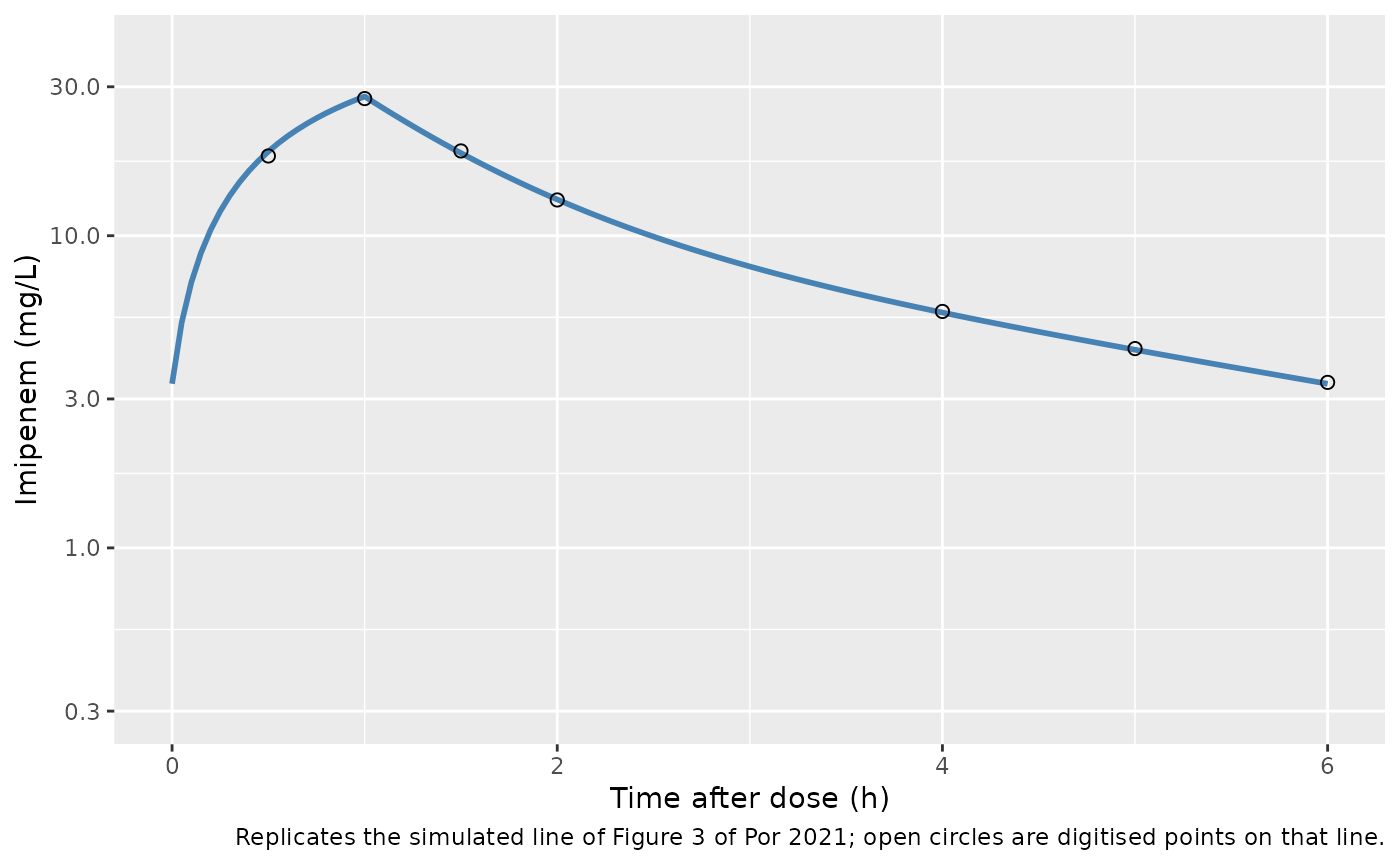
Figure 3: steady-state profile in the Boucher 2016 burn cohort
Figure 3 of Por 2021 overlays a simulated mean profile on data from Boucher 2016 after 1000 mg every 6 h as 1-h infusions at steady state, for weight 90 kg, albumin 3.2 g/dL and a CVVH clearance of 3.27 L/h. The simulated line was digitised by the maintainers from the published image (raster; about 3% reading error on the log axis). It coincides with the typical-value solve on the CVVH branch.
ev3 <- data.frame(
  id = 1L,
  time = c(0, seq(0, 6, by = 0.05)),
  evid = c(1L, rep(0L, 121)),
  amt = c(1000, rep(0, 121)),
  rate = c(1000, rep(0, 121)),
  ii = c(6, rep(0, 121)),
  ss = c(1L, rep(0L, 121)),
  cmt = "central",
  WT = 90, ALB = 32, CRCL = 100, RRT_CRRT_STATUS = 1, QEFF = 3.27
)
s3 <- rxode2::rxSolve(m0, ev3,
  returnType = "data.frame",
  rtol = 1e-10, atol = 1e-12, ssRtol = 1e-10, ssAtol = 1e-12, maxsteps = 1e6
)
#> ℹ omega/sigma items treated as zero: 'etalcl', 'etalvc'

fig3_dig <- tibble::tribble(
  ~time, ~Cc_fig,
  0.5, 18.01,
  1, 27.50,
  1.5, 18.69,
  2, 13.02,
  4, 5.72,
  5, 4.35,
  6, 3.39
)
fig3_cmp <- fig3_dig |>
  dplyr::mutate(
    Cc_sim = stats::approx(s3$time, s3$Cc, xout = time)$y,
    pct_diff = 100 * (Cc_sim / Cc_fig - 1)
  )
knitr::kable(fig3_cmp, digits = 2,
caption = "Typical-value solve vs the simulated line digitised from Figure 3.")| time | Cc_fig | Cc_sim | pct_diff |
|---|---|---|---|
| 0.5 | 18.01 | 18.61 | 3.35 |
| 1.0 | 27.50 | 27.93 | 1.55 |
| 1.5 | 18.69 | 18.39 | -1.59 |
| 2.0 | 13.02 | 13.07 | 0.35 |
| 4.0 | 5.72 | 5.67 | -0.80 |
| 5.0 | 4.35 | 4.31 | -0.87 |
| 6.0 | 3.39 | 3.36 | -1.02 |
stopifnot(
  nrow(fig3_cmp) == 7L,
  abs(stats::median(fig3_cmp$pct_diff)) < 3,
  max(abs(fig3_cmp$pct_diff)) < 8
)

ggplot(s3, aes(time, Cc)) +
  geom_line(colour = "steelblue", linewidth = 1) +
  geom_point(data = fig3_dig, aes(time, Cc_fig), shape = 1, size = 2) +
  scale_y_log10(limits = c(0.3, 40)) +
  labs(
    x = "Time after dose (h)", y = "Imipenem (mg/L)",
    caption = paste(
      "Replicates the simulated line of Figure 3 of Por 2021;",
      "open circles are digitised points on that line."
    )
  )
Figures 4 and 5: probability of target attainment
Por 2021 simulated 70-kg patients at steady state and defined target attainment as free concentration above the MIC for at least 40% of the dosing interval, with imipenem 20% protein bound. Normal renal function (NRF) was CrCl drawn uniformly from 100-130 mL/min and augmented renal clearance (ARC) from 150-250 mL/min. Figure 4 varies albumin as a surrogate for burn size (3.45-4, 2.6-3.15 and 1.5-2.2 g/dL for 0-10%, 25-50% and 70-100% TBSA); Figure 5 fixes albumin at 3 g/dL and adds a CVVH clearance of 0, 3 or 5 L/h.
The paper simulated 1000 patients per group; this article uses 200. The cohort covariates and random effects are drawn with base R and passed to the typical-value model as data, so the result is identical on every machine. Target attainment is computed on individual predictions without residual error.
n_arm <- 200
set.seed(20210901)
tgrid <- seq(0, 6, by = 0.05)

make_arm <- function(arm, dose, crcl, alb_gdL, qeff, id0) {
  subj <- data.frame(
    id = id0 + seq_len(n_arm),
    arm = arm,
    WT = 70,
    CRCL = stats::runif(n_arm, crcl[1], crcl[2]),
    ALB = 10 * stats::runif(n_arm, alb_gdL[1], alb_gdL[2]),
    RRT_CRRT_STATUS = 0,
    QEFF = qeff,
    etalcl = stats::rnorm(n_arm, 0, sqrt(0.093)),
    etalvc = stats::rnorm(n_arm, 0, sqrt(0.13))
  )
  dose_rows <- dplyr::mutate(subj,
    time = 0, evid = 1L, amt = dose, rate = dose, ii = 6, ss = 1L
  )
  obs_rows <- tidyr::crossing(subj, time = tgrid) |>
    dplyr::mutate(evid = 0L, amt = 0, rate = 0, ii = 0, ss = 0L)
  dplyr::bind_rows(dose_rows, obs_rows) |>
    dplyr::mutate(cmt = "central") |>
    dplyr::arrange(id, time, dplyr::desc(evid))
}

solve_arms <- function(ev) {
  # The random effects are supplied as data to the zeroRe() model, so
  # rxode2 draws nothing; muffle only its "no omega" notice.
  s <- withCallingHandlers(
    rxode2::rxSolve(m0, ev,
      returnType = "data.frame", keep = "arm",
      ssRtol = 1e-8, ssAtol = 1e-10, maxsteps = 1e6
    ),
    warning = function(w) {
      if (grepl("omega", conditionMessage(w))) invokeRestart("muffleWarning")
    }
  )
  stopifnot(!anyNA(s$Cc))
  s
}

pta_tab <- function(s, mics, dose_lab) {
  per_id <- s |>
    dplyr::filter(time < 6) |>
    dplyr::group_by(arm, id)
  dplyr::bind_rows(lapply(mics, function(m) {
    per_id |>
      dplyr::summarise(ft = mean(0.8 * Cc > m), .groups = "drop") |>
      dplyr::group_by(arm) |>
      dplyr::summarise(PTA = 100 * mean(ft >= 0.4), .groups = "drop") |>
      dplyr::mutate(MIC = m, dose = dose_lab)
  }))
}
mics <- c(0.5, 1, 2, 4, 8, 16)
Figure 4: renal function and burn size, 500 mg every 6 h
fig4_arms <- tibble::tribble(
  ~arm, ~crcl_lo, ~crcl_hi, ~alb_lo, ~alb_hi,
  "NRF, TBSA 0-10%", 100, 130, 3.45, 4,
  "NRF, TBSA 25-50%", 100, 130, 2.6, 3.15,
  "NRF, TBSA 70-100%", 100, 130, 1.5, 2.2,
  "ARC, TBSA 0-10%", 150, 250, 3.45, 4,
  "ARC, TBSA 25-50%", 150, 250, 2.6, 3.15,
  "ARC, TBSA 70-100%", 150, 250, 1.5, 2.2
)
ev4 <- dplyr::bind_rows(lapply(seq_len(nrow(fig4_arms)), function(i) {
  a <- fig4_arms[i, ]
  make_arm(a$arm, 500, c(a$crcl_lo, a$crcl_hi), c(a$alb_lo, a$alb_hi), 0, i * 1000)
}))
s4 <- solve_arms(ev4)
#> ℹ omega/sigma items treated as zero: 'etalcl', 'etalvc'
pta4 <- pta_tab(s4, mics, "500 mg q6h")

trough4 <- s4 |>
  dplyr::filter(abs(time - 6) < 1e-8) |>
  dplyr::group_by(arm) |>
  dplyr::summarise(
    `Median trough (mg/L)` = stats::median(Cc),
    `Trough > 5 mg/L (%)` = 100 * mean(Cc > 5),
    .groups = "drop"
  )

pta4 |>
  dplyr::filter(MIC %in% c(2, 4, 8)) |>
  tidyr::pivot_wider(names_from = MIC, values_from = PTA, names_prefix = "PTA MIC ") |>
  dplyr::left_join(trough4, by = "arm") |>
  dplyr::select(-dose) |>
  dplyr::rename(Group = arm) |>
knitr::kable(digits = 1, caption = "Simulated PTA (%) and troughs; compare Figure 4 of Por 2021.")| Group | PTA MIC 2 | PTA MIC 4 | PTA MIC 8 | Median trough (mg/L) | Trough > 5 mg/L (%) |
|---|---|---|---|---|---|
| ARC, TBSA 0-10% | 92.5 | 45.5 | 3.5 | 1.2 | 2.0 |
| ARC, TBSA 25-50% | 91.5 | 44.5 | 3.5 | 1.9 | 7.5 |
| ARC, TBSA 70-100% | 96.0 | 57.5 | 1.5 | 2.5 | 8.5 |
| NRF, TBSA 0-10% | 98.5 | 77.5 | 13.5 | 1.9 | 9.5 |
| NRF, TBSA 25-50% | 97.5 | 75.0 | 8.5 | 2.9 | 17.0 |
| NRF, TBSA 70-100% | 99.0 | 82.0 | 10.0 | 3.8 | 24.0 |
ggplot(pta4, aes(MIC, PTA, colour = arm)) +
  geom_line() +
  geom_point() +
  scale_x_log10(breaks = mics) +
  labs(
    x = "MIC (mg/L)", y = "PTA (%)", colour = NULL,
    caption = "Replicates Figure 4 (top) of Por 2021."
  )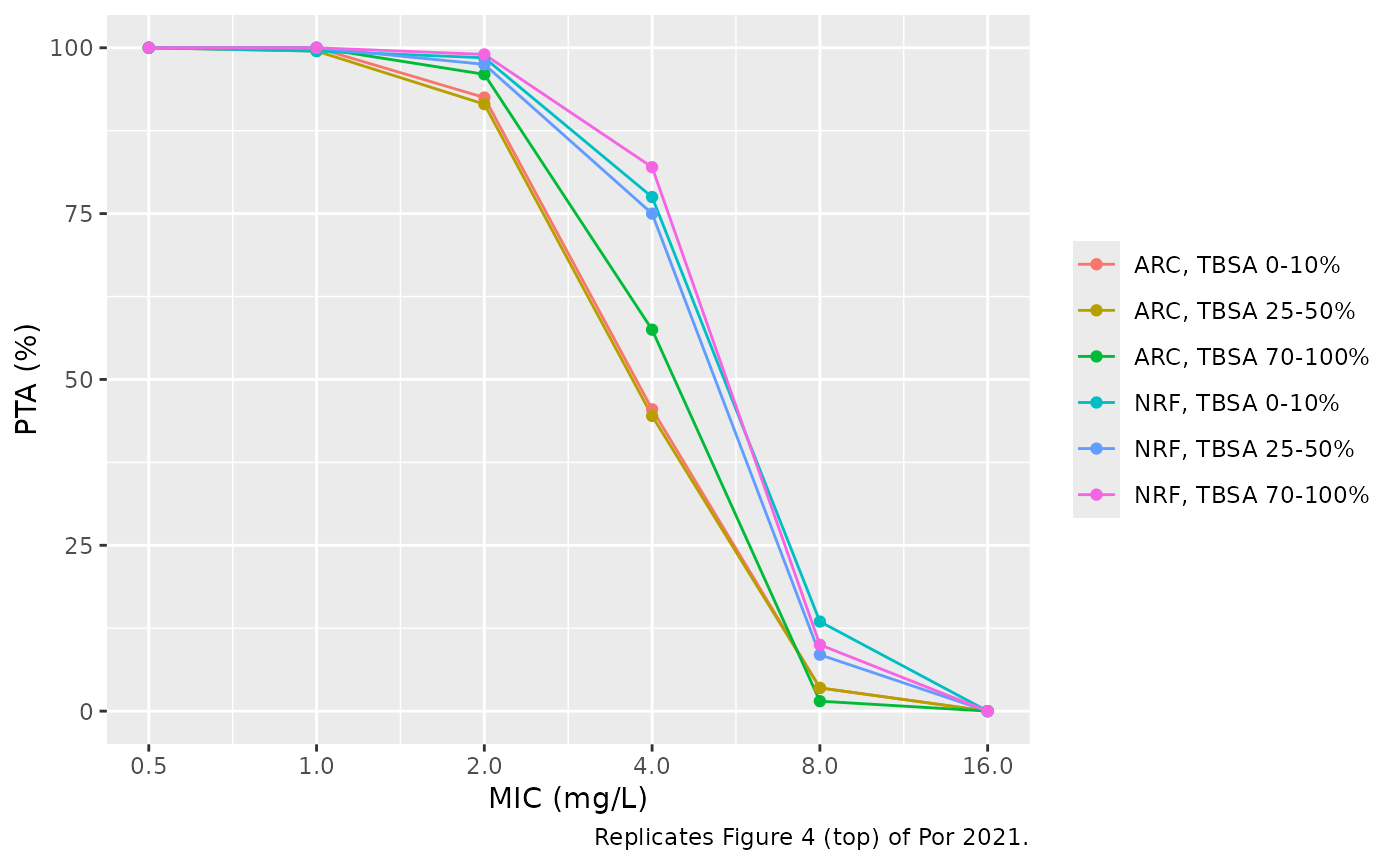
Por 2021 reports that 500 mg every 6 h attains an MIC of 2 mg/L (PTA above 80%) in every renal-function and burn-size group, and that the probability of a trough above 5 mg/L is highest, almost 20%, for NRF with 70-100% TBSA. Read by eye from Figure 4, PTA at an MIC of 4 mg/L is roughly 72-80% for the NRF groups and 42-55% for the ARC groups; the simulated group values fall within or a few points above those bands, and their pooled means are asserted below. The trough-above-5 mg/L percentages rest on a handful of subjects per 200-subject group, so they are shown but not asserted; the median trough, which moves with volume for every subject, is asserted instead.
p4 <- function(a, m) {
  v <- pta4$PTA[pta4$arm == a & pta4$MIC == m]
  if (length(v) != 1L) stop("no unique PTA row for ", a, " at MIC ", m)
  v
}
tr4 <- function(a) {
  v <- trough4$`Median trough (mg/L)`[trough4$arm == a]
  if (length(v) != 1L) stop("no unique trough row for ", a)
  v
}
nrf <- grep("^NRF", fig4_arms$arm, value = TRUE)
arc <- grep("^ARC", fig4_arms$arm, value = TRUE)
stopifnot(
  length(nrf) == 3L, length(arc) == 3L,
  # Text: MIC 2 attained (PTA > 80%) in every group.
  all(vapply(fig4_arms$arm, p4, numeric(1), m = 2) > 80),
  # MIC 4 bands read from Figure 4 (NRF about 72-80%, ARC about 42-55%),
  # pooled over the three burn-size groups.
  abs(mean(vapply(nrf, p4, numeric(1), m = 4)) - 75) < 10,
  abs(mean(vapply(arc, p4, numeric(1), m = 4)) - 47) < 10,
  # Larger burns (lower albumin, larger volumes) give higher troughs.
  tr4("NRF, TBSA 70-100%") > tr4("NRF, TBSA 0-10%"),
  tr4("ARC, TBSA 70-100%") > tr4("ARC, TBSA 0-10%")
)
Figure 5: renal function and CVVH intensity
Figure 5 simulates CVVH in patients whose kidneys are still working:
the NRF and ARC curves separate at every CVVH intensity. In this model
that scenario is the CrCl-driven clearance branch
(RRT_CRRT_STATUS = 0) with the haemofilter clearance added
through QEFF, exactly as in Equation 5. The CVVH branch
(RRT_CRRT_STATUS = 1) has no CrCl term and could not
separate NRF from ARC.
fig5_arms <- tidyr::crossing(
  renal = c("NRF", "ARC"),
  qeff = c(0, 3, 5),
  dose = c(500, 1000)
) |>
  dplyr::mutate(
    arm = paste0(
      renal, ", ", ifelse(qeff == 0, "no CVVH", paste("CVVH", qeff, "L per h")),
      ", ", dose, " mg"
    )
  )
ev5 <- dplyr::bind_rows(lapply(seq_len(nrow(fig5_arms)), function(i) {
  a <- fig5_arms[i, ]
  crcl <- if (a$renal == "NRF") c(100, 130) else c(150, 250)
  make_arm(a$arm, a$dose, crcl, c(3, 3), a$qeff, 100000 + i * 1000)
}))
s5 <- solve_arms(ev5)
#> ℹ omega/sigma items treated as zero: 'etalcl', 'etalvc'
pta5 <- pta_tab(s5, mics, NA_character_) |>
  dplyr::select(-dose) |>
  dplyr::left_join(fig5_arms, by = "arm")

pta5 |>
  dplyr::filter(MIC %in% c(2, 4, 8)) |>
  dplyr::select(dose, renal, qeff, MIC, PTA) |>
  tidyr::pivot_wider(names_from = MIC, values_from = PTA, names_prefix = "PTA MIC ") |>
  dplyr::arrange(dose, renal, qeff) |>
  dplyr::rename("Dose (mg q6h)" = dose, "Renal function" = renal, "CVVH CL (L/h)" = qeff) |>
knitr::kable(digits = 1, caption = "Simulated PTA (%); compare Figure 5 of Por 2021.")| Dose (mg q6h) | Renal function | CVVH CL (L/h) | PTA MIC 2 | PTA MIC 4 | PTA MIC 8 |
|---|---|---|---|---|---|
| 500 | ARC | 0 | 91.5 | 47.5 | 1.0 |
| 500 | ARC | 3 | 82.0 | 19.5 | 0.0 |
| 500 | ARC | 5 | 71.0 | 9.5 | 0.0 |
| 500 | NRF | 0 | 98.0 | 75.0 | 10.0 |
| 500 | NRF | 3 | 95.0 | 50.5 | 0.0 |
| 500 | NRF | 5 | 91.5 | 24.0 | 0.0 |
| 1000 | ARC | 0 | 100.0 | 91.5 | 40.5 |
| 1000 | ARC | 3 | 99.5 | 79.0 | 20.5 |
| 1000 | ARC | 5 | 98.5 | 73.5 | 8.5 |
| 1000 | NRF | 0 | 100.0 | 97.5 | 74.5 |
| 1000 | NRF | 3 | 99.5 | 92.5 | 44.0 |
| 1000 | NRF | 5 | 99.5 | 91.0 | 26.0 |
ggplot(pta5, aes(MIC, PTA,
  colour = factor(qeff), linetype = renal,
  group = interaction(renal, qeff)
)) +
  geom_line() +
  geom_point() +
  facet_wrap(~ paste(dose, "mg every 6 h"), ncol = 1) +
  scale_x_log10(breaks = mics) +
  labs(
    x = "MIC (mg/L)", y = "PTA (%)", colour = "CVVH CL (L/h)", linetype = NULL,
    caption = "Replicates Figure 5 of Por 2021."
  )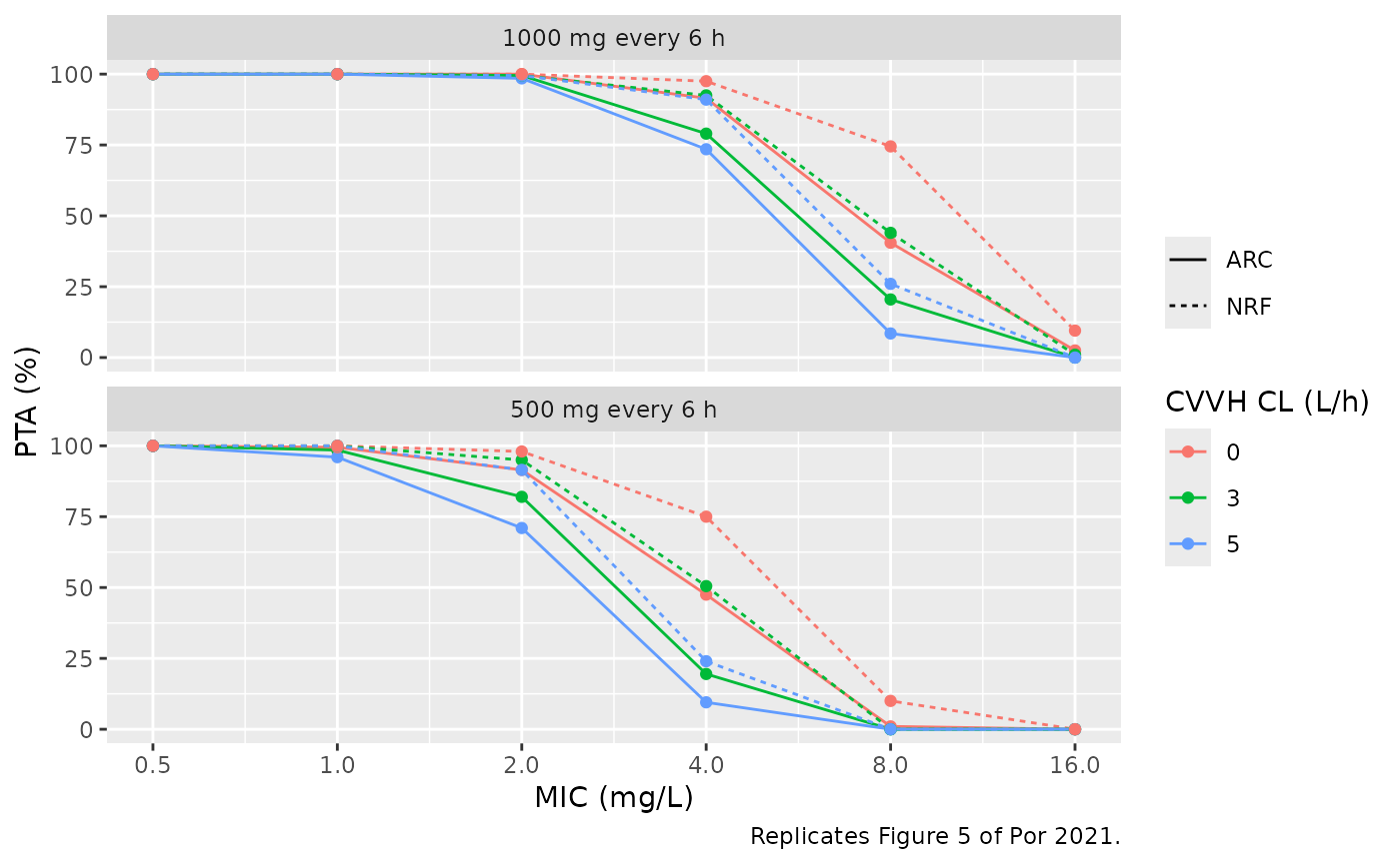
The paper’s text quotes, for 500 mg every 6 h at an MIC of 2 mg/L, a PTA of 90-98% except for ARC combined with 3-5 L/h CVVH (69-78%); and for 1000 mg every 6 h at an MIC of 4 mg/L, 89-98% except for ARC with CVVH (70-79%). The simulation reproduces both patterns. Its CVVH groups sit a few points above the figure, which is within what 200 subjects per group and a different random draw allow.
p5 <- function(renal, qeff, dose, m) {
  v <- pta5$PTA[pta5$renal == renal & pta5$qeff == qeff & pta5$dose == dose & pta5$MIC == m]
  if (length(v) != 1L) stop("no unique PTA row")
  v
}
others <- function(dose, m) {
  c(
    p5("NRF", 0, dose, m), p5("NRF", 3, dose, m), p5("NRF", 5, dose, m),
    p5("ARC", 0, dose, m)
  )
}
arc_cvvh <- function(dose, m) c(p5("ARC", 3, dose, m), p5("ARC", 5, dose, m))
stopifnot(
  # 500 mg, MIC 2: text 90-98% for the other groups, 69-78% for ARC + CVVH.
  min(others(500, 2)) > 85,
  abs(mean(arc_cvvh(500, 2)) - 73.5) < 10,
  # 1000 mg, MIC 4: text 89-98% for the other groups, 70-79% for ARC + CVVH.
  min(others(1000, 4)) > 85,
  abs(mean(arc_cvvh(1000, 4)) - 74.5) < 10,
  # ARC plus the most intense CVVH is the worst group in both panels.
  p5("ARC", 5, 500, 2) == min(pta5$PTA[pta5$dose == 500 & pta5$MIC == 2]),
  p5("ARC", 5, 1000, 4) == min(pta5$PTA[pta5$dose == 1000 & pta5$MIC == 4])
)
NCA of the steady-state interval (PKNCA)
Por 2021 reports no NCA table. The check below runs PKNCA on the
steady-state interval of the 500 mg Figure 5 groups and confirms the
steady-state identity AUCtau = Dose / CL subject by
subject, which tests that the haemofilter clearance really enters total
elimination.
conc5 <- s5 |>
  dplyr::filter(!is.na(Cc)) |>
  dplyr::inner_join(dplyr::distinct(fig5_arms, arm, dose), by = "arm") |>
  dplyr::filter(dose == 500) |>
  dplyr::select(arm, id, time, Cc, cl)
dose5 <- conc5 |>
  dplyr::distinct(arm, id) |>
  dplyr::mutate(time = 0, amt = 500)

conc_obj <- PKNCA::PKNCAconc(conc5, Cc ~ time | arm + id)
dose_obj <- PKNCA::PKNCAdose(dose5, amt ~ time | arm + id)
intervals <- data.frame(start = 0, end = 6, cmax = TRUE, cmin = TRUE, tmax = TRUE, auclast = TRUE)
nca <- PKNCA::pk.nca(PKNCA::PKNCAdata(conc_obj, dose_obj, intervals = intervals))
nca_df <- as.data.frame(nca)

nca_df |>
  dplyr::group_by(arm, PPTESTCD) |>
  dplyr::summarise(median = stats::median(PPORRES), .groups = "drop") |>
  tidyr::pivot_wider(names_from = PPTESTCD, values_from = median) |>
  dplyr::rename(
    Group = arm, "Cmax (mg/L)" = cmax, "Cmin (mg/L)" = cmin,
    "Tmax (h)" = tmax, "AUCtau (mg*h/L)" = auclast
  ) |>
knitr::kable(digits = 2, caption = "Median steady-state NCA, 500 mg every 6 h (1-h infusion).")| Group | AUCtau (mg*h/L) | Cmax (mg/L) | Cmin (mg/L) | Tmax (h) |
|---|---|---|---|---|
| ARC, CVVH 3 L per h, 500 mg | 27.22 | 13.60 | 1.32 | 1 |
| ARC, CVVH 5 L per h, 500 mg | 24.33 | 13.13 | 1.01 | 1 |
| ARC, no CVVH, 500 mg | 32.82 | 14.67 | 1.91 | 1 |
| NRF, CVVH 3 L per h, 500 mg | 33.20 | 14.85 | 1.98 | 1 |
| NRF, CVVH 5 L per h, 500 mg | 29.44 | 13.92 | 1.57 | 1 |
| NRF, no CVVH, 500 mg | 41.27 | 16.94 | 2.82 | 1 |
auc_chk <- nca_df |>
  dplyr::filter(PPTESTCD == "auclast") |>
  dplyr::inner_join(dplyr::distinct(conc5, arm, id, cl), by = c("arm", "id")) |>
  dplyr::mutate(rel_err = PPORRES * cl / 500 - 1)
# Same drawn parameters on both sides, so the only difference is the
# trapezoid on a 0.05-h grid: a tight bound is correct here.
stopifnot(
  nrow(auc_chk) == 6L * n_arm,
  max(abs(auc_chk$rel_err)) < 0.01
)
Assumptions and deviations
- Residual error scale. Table 2 prints the proportional error as 0.3 without saying whether it is a standard deviation or a variance. It is read as a standard deviation (30%): Table S2 reports the additive error of the preceding model in mg/L, which is the unit of a standard deviation, and prints the proportional error beside it in the same way.
-
Haemofilter clearance is a covariate.
QEFFis each patient’s measuredQf x Sc x CF(Equations 1-3). Set it to 0 for a patient not on CVVH. It is not switched off byRRT_CRRT_STATUS, because Equation 5 adds it unconditionally and because Figure 5 combines it with the CrCl-driven branch. -
CRCLmust be supplied for CVVH patients even though it has no effect there; a missing value would propagate through the clearance expression. -
Albumin units. The model was fitted on albumin in
g/dL; the canonical
ALBcolumn is g/L and is divided by 10 insidemodel(). The fitted albumin range was 1.5-3.5 g/dL, so the Table 3 “healthy” predictions at 4 g/dL are extrapolations, as the paper acknowledges by reporting a 30-60% error for Vp in those populations. - Table 3 renal-impairment row. Weight and creatinine clearance are transposed in the published row (see the Table 3 check above).
- Figure 4 infusion duration. The caption does not state it; 1 h is used, as stated for Figure 5.
- Figure 5 albumin. The caption gives 3 g/dL for 30% TBSA, the text 3.2 g/dL. The caption value is used; by Figure 1 (albumin = 3.68 - 0.021 x TBSA) 30% TBSA corresponds to 3.05 g/dL.
- Cohort size. 200 simulated patients per group instead of 1000.