Ceftazidime/avibactam + colistin against KPC-3 Klebsiella pneumoniae (Aubry 2023)
Source:vignettes/articles/Aubry_2023_ceftazidime_avibactam_colistin.Rmd
Aubry_2023_ceftazidime_avibactam_colistin.RmdModel and source
- Article: https://doi.org/10.1128/aac.00301-23
- Supplementary material (
aac.00301-23-s0001.docx): visual predictive checks for the three other isolates (Figs. S1-S3), observed-versus-predicted plots, and the NONMEM control streams of the expected-additivity (Code S1) and observed-interaction (Code S2) models for isolate NARA1295.
isolates <- c("NARA1295", "NARA1584", "NARA1182", "NARA864")
model_names <- paste0("Aubry_2023_ceftazidime_avibactam_colistin_", isolates)
mods <- setNames(lapply(model_names, function(nm) rxode2::rxode2(readModelDb(nm))), isolates)
cat(mods$NARA1295$reference, sep = "\n")
#> Aubry R, Buyck J, Prouvensier L, Decousser JW, Nordmann P, Wicha SG, Marchand S, Gregoire N. An improved PKPD modeling approach to characterize the pharmacodynamic interaction over time between ceftazidime/avibactam and colistin from in vitro time-kill experiments against multidrug-resistant Klebsiella pneumoniae isolates. Antimicrob Agents Chemother. 2023;67(10):e00301-23. doi:10.1128/aac.00301-23. Structural equations: main-text Eqs 1-6 and the NONMEM control stream of this isolate's observed interaction model (Supplementary Code S2). Parameter estimates: main-text Table 2.
Aubry 2023 fits one semi-mechanistic time-kill model per isolate to static time-kill curves of four KPC-3-producing Klebsiella pneumoniae clinical isolates exposed to ceftazidime/avibactam (CZA; avibactam always at 4 mg/L) and colistin (CST), alone and in combination. The structure is shared, but every isolate has its own parameter column in Table 2 and its own visual predictive check, so the library ships four models:
| Model | Isolate | GPDI interaction (colistin as perpetrator) |
|---|---|---|
Aubry_2023_ceftazidime_avibactam_colistin_NARA1295 |
NARA1295 (ST512) | lowers the CZA EC50 by up to 51.4% |
Aubry_2023_ceftazidime_avibactam_colistin_NARA1584 |
NARA1584 (ST101) | lowers the CZA EC50 by up to 48.3% |
Aubry_2023_ceftazidime_avibactam_colistin_NARA1182 |
NARA1182 (ST512) | lowers the CZA EC50 by up to 48.6% |
Aubry_2023_ceftazidime_avibactam_colistin_NARA864 |
NARA864 (ST348) | lowers the CZA Emax by up to 65.8% |
Each model has:
- one homogeneous bacterial population
cfu(CFU/mL) with logistic growth towardbmax; - a sigmoidal Emax kill by each drug, whose Emax falls in proportion
to the fraction of bacteria in an “adapted” state
(
aron_caz,aron_col) – an empirical two-state adaptive-resistance model per drug, switched on only while that drug is present, with no reversal (koff = 0); - Bliss independence as the additivity criterion, with each kill rate normalised by the larger of the two mono-drug Emax values (Code S2);
- a general pharmacodynamic interaction (GPDI) term through which colistin modifies one ceftazidime parameter;
- the observation
log_cfu= log10 CFU/mL with an additive residual error.
Drug concentrations are supplied as the covariates
CONC_CAZ_MGL and CONC_CST_MGL. There is no PK
and there are no dosing events: the solver integrates the bacterial and
adaptation states from the inoculum. This is a pharmacodynamic model of
an in vitro experiment, so PKNCA is not the right validation target; the
checks below compare the model against the paper’s own model predictions
instead.
Population (biological context)
pop <- lapply(mods, function(m) m$population)
data.frame(
  isolate = isolates,
  disease_state = vapply(pop, function(p) p$disease_state, character(1)),
  inoculum = vapply(pop, function(p) p$initial_inoculum, character(1))
) |>
knitr::kable()| isolate | disease_state | inoculum | |
|---|---|---|---|
| NARA1295 | NARA1295 | Clinical K. pneumoniae isolate from the human strain collection (2019-2021) of the National Reference Center for Emerging Antibiotic Resistance (NARA, Fribourg, Switzerland). Sequence type ST512; resistance genes KPC-3, SHV-11 (35Q), TEM-1D, truncated OmpK35 (25%) and OmpK36 with a glycine-aspartate insertion (Table 1). MICs (broth microdilution, EUCAST): ceftazidime/avibactam 8 mg/L (avibactam fixed at 4 mg/L), colistin 0.125 mg/L; susceptible to both. | Estimated 10^5.63 CFU/mL (Table 2) |
| NARA1584 | NARA1584 | Clinical K. pneumoniae isolate from the human strain collection (2019-2021) of the National Reference Center for Emerging Antibiotic Resistance (NARA, Fribourg, Switzerland). Sequence type ST101; resistance genes KPC-3, SHV-1, truncated OmpK35 (17%) and OmpK36 with a threonine-aspartate insertion (Table 1). MICs (broth microdilution, EUCAST): ceftazidime/avibactam 8 mg/L (avibactam fixed at 4 mg/L), colistin 0.125 mg/L; susceptible to both. | Estimated 10^5.62 CFU/mL (Table 2) |
| NARA1182 | NARA1182 | Clinical K. pneumoniae isolate from the human strain collection (2019-2021) of the National Reference Center for Emerging Antibiotic Resistance (NARA, Fribourg, Switzerland). Sequence type ST512; resistance genes KPC-3, SHV-11 (35Q), truncated OmpK35 (25%) and OmpK36 with a glycine-aspartate insertion (Table 1). MICs (broth microdilution, EUCAST): ceftazidime/avibactam 4 mg/L (avibactam fixed at 4 mg/L), colistin 0.125 mg/L; susceptible to both. | Estimated 10^5.53 CFU/mL (Table 2) |
| NARA864 | NARA864 | Clinical K. pneumoniae isolate from the human strain collection (2019-2021) of the National Reference Center for Emerging Antibiotic Resistance (NARA, Fribourg, Switzerland). Sequence type ST348; resistance genes KPC-3, SHV-11 (35Q), TEM-1D and OXA-9, with no porin alteration reported (Table 1). MICs (broth microdilution, EUCAST): ceftazidime/avibactam 2 mg/L (avibactam fixed at 4 mg/L), colistin 0.25 mg/L; susceptible to both. | Estimated 10^5.68 CFU/mL (Table 2) |
All four isolates come from the 2019-2021 human strain collection of the National Reference Center for Emerging Antibiotic Resistance (NARA, Fribourg, Switzerland) and are susceptible to both drugs (Table 1: CZA MICs 2-8 mg/L, CST MICs 0.125-0.25 mg/L). Static time-kill experiments ran for 30 h at 35 degrees C in 10 mL cation-adjusted Mueller-Hinton broth II from an inoculum of about 5 x 10^5 CFU/mL, with counts at 0, 2, 4, 8, 24 and 30 h and a lower limit of quantification of 200 CFU/mL (2.3 log10 CFU/mL).
Source trace
| Element | Source location | Value(s) in the files |
|---|---|---|
| Sigmoidal Emax kill | Eq 1 |
emax_*, ec50_*, hill_*
|
| Two-state adaptive resistance | Eqs 2-3; Code S2 DADT(4)-DADT(7)
|
aron_* / aroff_*, kon_*,
koff
|
| Emax reduced by the adapted fraction | Eq 4; Code S2 E_ADAPT_CZA = AR_CZA*A(4)
|
armax_* |
| Adaptation only while the drug is present | Code S2 IF(A(1).GT.0) ADAPT_CZA=KON_CZA
|
kon_*_i <- kon_* * (CONC > 0) |
| Logistic growth on the linear CFU scale | Eq 5; Code S2 DADT(3),
A_0(3)=10**INOC
|
kg, log10bmax, log10inoc
|
| Bliss independence, normalised by max Emax | Code S2 E_COMB
|
emax_norm, kill_comb
|
| GPDI interaction | Eq 6; Code S2 INTERACTION
|
int_col_caz, ec50int_col_caz,
hillint_col_caz
|
| Victim parameter (EC50 vs Emax) | Table 2 rows INT_EC50 / INT_Emax;
Results |
EC50 for NARA1295/1584/1182, Emax for NARA864 |
| Residual error | Table 2 RES_ADD; Code S2
W = SQRT(SIGMA(1))
|
addSd = sqrt(RES_ADD) (see below) |
| Observation floor | Code S2 IF(BTOT_ERR<1e-6) BTOT_ERR=1e-6
|
log10(max(cfu, 1e-6)) |
| All parameter estimates | Table 2 (one column per isolate) |
ini() of each file |
Parameter tables (paper vs. file)
Table 2 is transcribed below in the paper’s units (percentages for
ARmax and INT, the residual entry as printed).
The file values are read from each model’s ini() and
converted to the same units, so the comparison checks the transcription
and every back-transform in one pass.
table2 <- read.csv(text = "
parameter,NARA1295,NARA1584,NARA1182,NARA864
INOC,5.63,5.62,5.53,5.68
KG,1.40,1.77,1.78,1.84
Bmax,8.80,9.13,8.43,9.01
Emax_CZA,4.59,6.27,7.51,9.17
EC50_CZA,13.39,13.47,2.51,0.46
gamma_CZA,2.13,1.84,1.53,1.79
KON_CZA,0.24,0.32,0.36,0.66
KOFF,0,0,0,0
ARmax_CZA,71.9,73.0,78.6,82.5
Emax_CST,13.12,8.78,14.31,8.81
EC50_CST,0.60,0.33,0.33,0.21
gamma_CST,0.96,1.13,1.21,1.16
KON_CST,0.65,0.52,1.18,0.75
ARmax_CST,91.8,83.1,87.0,80.3
INT,-51.4,-48.3,-48.6,-65.8
EC50_INT,0.06,0.06,0.07,0.39
gamma_INT,10,10,10,1
RES_ADD,1.74,1.01,1.44,2.25
")

file_values <- function(m) {
  th <- m$theta
  c(
    INOC = th[["log10inoc"]], KG = th[["kg"]], Bmax = th[["log10bmax"]],
    Emax_CZA = th[["emax_caz"]], EC50_CZA = th[["ec50_caz"]],
    gamma_CZA = th[["hill_caz"]], KON_CZA = th[["kon_caz"]], KOFF = th[["koff"]],
    ARmax_CZA = 100 * th[["armax_caz"]],
    Emax_CST = th[["emax_col"]], EC50_CST = th[["ec50_col"]],
    gamma_CST = th[["hill_col"]], KON_CST = th[["kon_col"]],
    ARmax_CST = 100 * th[["armax_col"]],
    INT = 100 * th[["int_col_caz"]], EC50_INT = th[["ec50int_col_caz"]],
    gamma_INT = th[["hillint_col_caz"]],
    # Table 2 prints the $SIGMA variance; the file carries its square root.
    RES_ADD = th[["addSd"]]^2
  )
}
cmp <- table2 |>
  pivot_longer(-parameter, names_to = "isolate", values_to = "paper") |>
  mutate(file = mapply(function(p, i) file_values(mods[[i]])[[p]], parameter, isolate))
stopifnot(all(abs(cmp$file - cmp$paper) < 1e-8))
cmp |>
  pivot_wider(names_from = isolate, values_from = c(paper, file)) |>
  select(parameter, ends_with("NARA1295"), ends_with("NARA1584"),
         ends_with("NARA1182"), ends_with("NARA864")) |>
knitr::kable(digits = 3)| parameter | paper_NARA1295 | file_NARA1295 | paper_NARA1584 | file_NARA1584 | paper_NARA1182 | file_NARA1182 | paper_NARA864 | file_NARA864 |
|---|---|---|---|---|---|---|---|---|
| INOC | 5.63 | 5.63 | 5.62 | 5.62 | 5.53 | 5.53 | 5.68 | 5.68 |
| KG | 1.40 | 1.40 | 1.77 | 1.77 | 1.78 | 1.78 | 1.84 | 1.84 |
| Bmax | 8.80 | 8.80 | 9.13 | 9.13 | 8.43 | 8.43 | 9.01 | 9.01 |
| Emax_CZA | 4.59 | 4.59 | 6.27 | 6.27 | 7.51 | 7.51 | 9.17 | 9.17 |
| EC50_CZA | 13.39 | 13.39 | 13.47 | 13.47 | 2.51 | 2.51 | 0.46 | 0.46 |
| gamma_CZA | 2.13 | 2.13 | 1.84 | 1.84 | 1.53 | 1.53 | 1.79 | 1.79 |
| KON_CZA | 0.24 | 0.24 | 0.32 | 0.32 | 0.36 | 0.36 | 0.66 | 0.66 |
| KOFF | 0.00 | 0.00 | 0.00 | 0.00 | 0.00 | 0.00 | 0.00 | 0.00 |
| ARmax_CZA | 71.90 | 71.90 | 73.00 | 73.00 | 78.60 | 78.60 | 82.50 | 82.50 |
| Emax_CST | 13.12 | 13.12 | 8.78 | 8.78 | 14.31 | 14.31 | 8.81 | 8.81 |
| EC50_CST | 0.60 | 0.60 | 0.33 | 0.33 | 0.33 | 0.33 | 0.21 | 0.21 |
| gamma_CST | 0.96 | 0.96 | 1.13 | 1.13 | 1.21 | 1.21 | 1.16 | 1.16 |
| KON_CST | 0.65 | 0.65 | 0.52 | 0.52 | 1.18 | 1.18 | 0.75 | 0.75 |
| ARmax_CST | 91.80 | 91.80 | 83.10 | 83.10 | 87.00 | 87.00 | 80.30 | 80.30 |
| INT | -51.40 | -51.40 | -48.30 | -48.30 | -48.60 | -48.60 | -65.80 | -65.80 |
| EC50_INT | 0.06 | 0.06 | 0.06 | 0.06 | 0.07 | 0.07 | 0.39 | 0.39 |
| gamma_INT | 10.00 | 10.00 | 10.00 | 10.00 | 10.00 | 10.00 | 1.00 | 1.00 |
| RES_ADD | 1.74 | 1.74 | 1.01 | 1.01 | 1.44 | 1.44 | 2.25 | 2.25 |
For NARA864 the interaction row is INT_Emax /
EC50_INT_Emax / gamma_INT_Emax; for the other
three it is INT_EC50 / EC50_INT_EC50 /
gamma_INT_EC50. The NARA864 growth rate, all interaction
Hill coefficients, the NARA864 interaction EC50 and KOFF
were not estimated (Table 2 “fixed”) and are wrapped in
fixed().
Simulation helpers
grid_events <- function(panels, times) {
  panels$id <- seq_len(nrow(panels))
  ev <- merge(panels, data.frame(time = times))
  ev$CONC_CAZ_MGL <- ev$caz
  ev$CONC_CST_MGL <- ev$col
  # Observations on the bacterial ODE state; log_cfu is returned alongside.
  ev$evid <- 0
  ev$cmt <- "cfu"
  dplyr::arrange(ev, id, time)
}
# The models have no between-tube variability, and each `id` is a
# drug-concentration scenario, not a subject. rxode2 warns about a
# multi-subject solve without omega; only that message is muffled.
muffle_no_omega <- function(w) {
  if (grepl("multi-subject simulation without", conditionMessage(w), fixed = TRUE)) {
    invokeRestart("muffleWarning")
  }
}
solve_typical <- function(mod, panels, times = seq(0, 30, by = 0.25)) {
  ev <- grid_events(panels, times)
  withCallingHandlers(
    rxode2::rxSolve(rxode2::zeroRe(mod, "sigma"), ev, omega = NA,
                    keep = c("caz", "col"), returnType = "data.frame"),
    warning = muffle_no_omega
  )
}
Carrying capacity and inoculum
With no drug the model is a pure logistic growth curve: it starts at
10^INOC and settles at 10^Bmax. A
mis-transcribed log10bmax or a missed 10^
back-transform shows up here immediately.
gc <- bind_rows(lapply(isolates, function(i) {
  solve_typical(mods[[i]], data.frame(caz = 0, col = 0), times = c(0, 30)) |>
    mutate(isolate = i)
}))
gc_chk <- gc |>
  select(isolate, time, log_cfu) |>
  pivot_wider(names_from = time, values_from = log_cfu, names_prefix = "t") |>
  mutate(
    inoc = vapply(isolate, function(i) mods[[i]]$theta[["log10inoc"]], numeric(1)),
    bmax = vapply(isolate, function(i) mods[[i]]$theta[["log10bmax"]], numeric(1))
  )
knitr::kable(gc_chk, digits = 3)| isolate | t0 | t30 | inoc | bmax |
|---|---|---|---|---|
| NARA1295 | 5.63 | 8.80 | 5.63 | 8.80 |
| NARA1584 | 5.62 | 9.13 | 5.62 | 9.13 |
| NARA1182 | 5.53 | 8.43 | 5.53 | 8.43 |
| NARA864 | 5.68 | 9.01 | 5.68 | 9.01 |
Mass balance of the adaptation states
aron + aroff is a fraction of the population and must
stay at 1 for each drug. The adaptation switch must also stay off for a
drug that is absent.
ab <- solve_typical(mods$NARA1295, data.frame(caz = c(8, 0), col = c(0, 0.25)))
stopifnot(
  all(abs(ab$aron_caz + ab$aroff_caz - 1) < 1e-6),
  all(abs(ab$aron_col + ab$aroff_col - 1) < 1e-6),
  # colistin-free arm: no colistin adaptation; CZA-free arm: no CZA adaptation
  max(ab$aron_col[ab$col == 0]) < 1e-9,
  max(ab$aron_caz[ab$caz == 0]) < 1e-9
)
# kon_caz = 0.24 1/h, so 1 - exp(-0.24 * 30) of the bacteria are adapted by 30 h
ab |>
  filter(time == 30) |>
  select(caz, col, aron_caz, aron_col) |>
  mutate(aron_caz_closed_form = ifelse(caz > 0, 1 - exp(-0.24 * 30), 0)) |>
knitr::kable(digits = 4)| caz | col | aron_caz | aron_col | aron_caz_closed_form |
|---|---|---|---|---|
| 8 | 0.00 | 0.9993 | 0 | 0.9993 |
| 0 | 0.25 | 0.0000 | 1 | 0.0000 |
Replicate the visual predictive checks (Figure 3, Figures S1-S3)
The models have no random effect except the residual error, and that
error is additive and symmetric on the log10 scale. The median of the
paper’s VPC simulations is therefore the typical prediction itself, so
the red median lines of the VPCs are a direct, quantitative target for
zeroRe() simulations.
The median lines of Figs. S1-S3 (high-resolution images in the supplement) were digitised by the maintainers from the image pixels: the y axis was calibrated on the printed 0.0 and 10.0 log10 CFU/mL ticks of each panel row, the x axis on the 0-30 h tick marks of each panel column, and the median was read at the six sampling times. Fig. 3 (NARA1295) is published only as a low-resolution image in which the median line could not be traced reliably, so NARA1295 is shown without digitised points; its grid of concentrations is the same as that of NARA1584.
# Digitised VPC medians (log10 CFU/mL) at 2, 4, 8, 24 and 30 h; caz and col
# are the ceftazidime and colistin concentrations (mg/L) of each panel.
dig <- read.csv(text = "
isolate,caz,col,t2,t4,t8,t24,t30
NARA1584,0,0,7.11,8.36,9.01,9.01,9.08
NARA1584,2,0,6.9,8.22,9.04,9.04,9.01
NARA1584,4,0,6.6,7.79,8.99,9.01,9.01
NARA1584,8,0,5.87,6.55,8.36,8.92,9.01
NARA1584,16,0,4.58,4.37,5.0,8.64,8.73
NARA1584,32,0,3.62,2.44,2.11,4.08,4.93
NARA1584,64,0,3.03,1.78,1.13,1.5,1.9
NARA1584,0,0.03,6.83,8.09,9.05,9.08,9.08
NARA1584,2,0.03,6.69,7.78,9.01,9.08,9.08
NARA1584,4,0.03,6.36,7.45,8.96,9.03,9.01
NARA1584,8,0.03,5.67,6.26,7.87,8.96,9.01
NARA1584,16,0.03,4.35,4.04,4.54,8.49,8.58
NARA1584,32,0.03,3.4,2.2,1.91,3.14,3.83
NARA1584,0,0.06,6.48,7.6,9.0,9.14,9.14
NARA1584,2,0.06,6.29,7.26,8.9,9.0,9.0
NARA1584,4,0.06,5.88,6.6,8.55,9.0,9.0
NARA1584,8,0.06,4.95,5.12,6.21,8.88,8.93
NARA1584,16,0.06,3.79,2.98,2.79,5.45,6.5
NARA1584,32,0.06,3.02,1.55,0.98,0.79,1.0
NARA1584,0,0.125,5.91,6.67,8.63,9.01,9.01
NARA1584,2,0.125,5.53,6.1,7.97,8.94,8.94
NARA1584,4,0.125,4.92,5.04,6.22,8.82,8.87
NARA1584,8,0.125,3.88,3.12,3.14,6.08,7.16
NARA1584,16,0.125,2.96,1.58,0.5,0.43,0.5
NARA1584,32,0.125,2.7,0.78,NA,NA,NA
NARA1584,0,0.25,4.95,5.38,7.02,8.92,8.94
NARA1584,2,0.25,4.69,4.88,6.17,8.83,8.87
NARA1584,4,0.25,4.18,3.94,4.58,8.59,8.66
NARA1584,8,0.25,3.29,2.18,1.78,3.1,3.66
NARA1584,16,0.25,2.51,0.82,NA,NA,NA
NARA1584,32,0.25,2.3,0.28,NA,NA,NA
NARA1584,0,0.5,3.97,3.8,4.88,8.78,8.8
NARA1584,0,1,3.05,2.56,3.12,7.16,8.31
NARA1584,0,2,2.46,1.74,1.95,4.95,5.99
NARA1584,0,4,2.18,1.22,1.24,3.64,4.51
NARA1182,0,0,6.85,8.17,8.33,8.38,8.38
NARA1182,1,0,5.96,6.83,8.24,8.31,8.31
NARA1182,2,0,4.98,5.09,6.5,8.15,8.17
NARA1182,4,0,3.64,3.12,3.45,7.58,7.89
NARA1182,8,0,2.79,1.69,1.29,3.52,4.61
NARA1182,16,0,2.32,0.94,0.28,1.48,2.11
NARA1182,0,0.03,6.74,7.99,8.32,8.42,8.37
NARA1182,1,0.03,5.72,6.57,8.06,8.23,8.23
NARA1182,2,0.03,4.78,4.78,6.08,8.16,8.23
NARA1182,4,0.03,3.5,2.84,2.98,6.81,7.77
NARA1182,8,0.03,2.6,1.39,0.78,2.65,3.4
NARA1182,0,0.06,6.33,7.64,8.4,8.43,8.43
NARA1182,1,0.06,5.43,6.07,7.69,8.26,8.29
NARA1182,2,0.06,4.36,4.29,5.19,8.14,8.21
NARA1182,4,0.06,3.17,2.36,2.29,5.14,6.29
NARA1182,8,0.06,2.36,0.95,0.14,1.1,1.57
NARA1182,0,0.125,5.74,6.83,8.18,8.3,8.3
NARA1182,1,0.125,4.0,3.83,4.49,7.99,8.01
NARA1182,2,0.125,2.88,1.91,1.63,3.52,4.26
NARA1182,4,0.125,1.99,0.57,NA,NA,NA
NARA1182,8,0.125,1.58,0.21,NA,NA,NA
NARA1182,0,0.25,4.81,5.38,7.02,8.15,8.17
NARA1182,1,0.25,3.12,2.56,2.82,5.33,6.09
NARA1182,2,0.25,2.18,1.01,NA,NA,NA
NARA1182,4,0.25,1.41,0.28,NA,NA,NA
NARA1182,8,0.25,1.03,NA,NA,NA,NA
NARA1182,0,0.5,3.62,3.83,4.77,7.93,7.89
NARA1182,0,1,2.68,2.54,2.91,5.02,5.63
NARA1182,0,2,2.11,1.62,1.74,2.37,2.61
NARA1182,0,4,1.81,1.2,1.2,1.15,1.13
NARA864,0,0,7.22,8.47,8.92,8.97,8.97
NARA864,0.25,0,5.95,6.98,8.73,8.86,8.89
NARA864,0.5,0,4.6,4.87,6.35,8.65,8.65
NARA864,1,0,3.28,2.86,3.52,7.35,8.25
NARA864,2,0,2.67,1.93,2.17,4.47,5.36
NARA864,4,0,2.3,1.53,1.67,3.54,4.21
NARA864,8,0,2.49,1.46,1.51,3.2,3.81
NARA864,16,0,2.25,1.35,1.56,3.1,3.65
NARA864,0,0.03,6.72,8.04,8.81,8.94,8.97
NARA864,0.25,0.03,5.58,6.4,8.28,8.81,8.81
NARA864,0.5,0.03,4.29,4.55,5.77,8.62,8.65
NARA864,1,0.03,3.28,2.78,3.25,6.53,7.54
NARA864,2,0.03,2.67,1.83,2.01,3.76,4.48
NARA864,4,0.03,2.33,1.61,1.59,2.94,3.41
NARA864,0,0.06,6.32,7.35,8.78,8.89,8.89
NARA864,0.25,0.06,5.34,5.95,7.67,8.73,8.73
NARA864,0.5,0.06,4.15,4.18,5.24,8.54,8.57
NARA864,1,0.06,3.17,2.62,2.96,5.45,6.35
NARA864,2,0.06,2.67,1.72,1.72,2.96,3.37
NARA864,4,0.06,2.3,1.48,1.35,2.06,2.38
NARA864,0,0.125,5.71,6.38,8.23,8.81,8.81
NARA864,0.25,0.125,4.79,5.11,6.48,8.73,8.73
NARA864,0.5,0.125,3.76,3.65,4.31,7.88,8.41
NARA864,1,0.125,2.91,2.25,2.25,3.81,4.13
NARA864,2,0.125,2.65,1.61,1.35,1.59,1.67
NARA864,4,0.125,2.35,1.32,1.01,0.79,0.71
NARA864,0,0.25,4.77,5.04,6.4,8.72,8.72
NARA864,0.25,0.25,4.19,4.03,4.85,8.51,8.56
NARA864,0.5,0.25,3.28,2.91,3.12,5.15,5.88
NARA864,1,0.25,2.77,1.87,1.6,1.6,1.52
NARA864,2,0.25,2.48,1.28,0.69,NA,NA
NARA864,4,0.25,2.24,1.07,0.45,NA,NA
NARA864,0,0.5,3.95,3.84,4.69,8.21,8.48
NARA864,0.25,0.5,3.49,3.04,3.39,5.92,6.72
NARA864,0.5,0.5,2.83,2.19,2.08,2.56,2.8
NARA864,1,0.5,2.45,1.36,0.91,NA,NA
NARA864,2,0.5,2.4,0.96,0.32,NA,NA
NARA864,4,0.5,2.05,0.83,NA,NA,NA
NARA864,0,1,3.33,3.02,3.33,5.71,6.67
NARA864,0,2,2.99,2.45,2.6,4.14,4.69
NARA864,0,4,2.8,2.22,2.17,3.25,3.65
NARA864,0,8,2.64,2.08,2.08,2.93,3.12
")
dig_long <- dig |>
  pivot_longer(starts_with("t"), names_to = "time", values_to = "log_cfu_paper",
               names_prefix = "t", names_transform = as.numeric) |>
  filter(!is.na(log_cfu_paper))
nrow(dig_long)
#> [1] 499
grid_1584 <- dig |> filter(isolate == "NARA1584") |> select(caz, col)
panels <- list(
  NARA1295 = grid_1584,
  NARA1584 = grid_1584,
  NARA1182 = dig |> filter(isolate == "NARA1182") |> select(caz, col),
  NARA864  = dig |> filter(isolate == "NARA864")  |> select(caz, col)
)
typ <- bind_rows(lapply(isolates, function(i) {
  solve_typical(mods[[i]], panels[[i]]) |> mutate(isolate = i)
}))
plot_isolate <- function(i, fig) {
  d <- typ |> filter(isolate == i)
  p <- ggplot(d, aes(time, log_cfu)) +
    geom_hline(yintercept = log10(200), linetype = "dashed", colour = "grey50") +
    geom_line(colour = "firebrick") +
    facet_grid(col ~ caz, labeller = label_both) +
    coord_cartesian(ylim = c(0, 10.5)) +
    scale_x_continuous(breaks = c(0, 8, 24)) +
    labs(x = "Time (h)", y = "log10 CFU/mL",
         title = paste0(i, ": typical prediction (line)",
                        if (i != "NARA1295") " vs digitised VPC median (points)"),
         caption = paste0("Replicates ", fig, " of Aubry 2023.\nColumns: ceftazidime (mg/L, ",
                          "with 4 mg/L avibactam); rows: colistin (mg/L). Dashed: LLOQ."))
  if (i != "NARA1295") {
    p <- p + geom_point(data = dig_long |> filter(isolate == i),
                        aes(time, log_cfu_paper), size = 0.8)
  }
  p
}
plot_isolate("NARA1295", "Figure 3")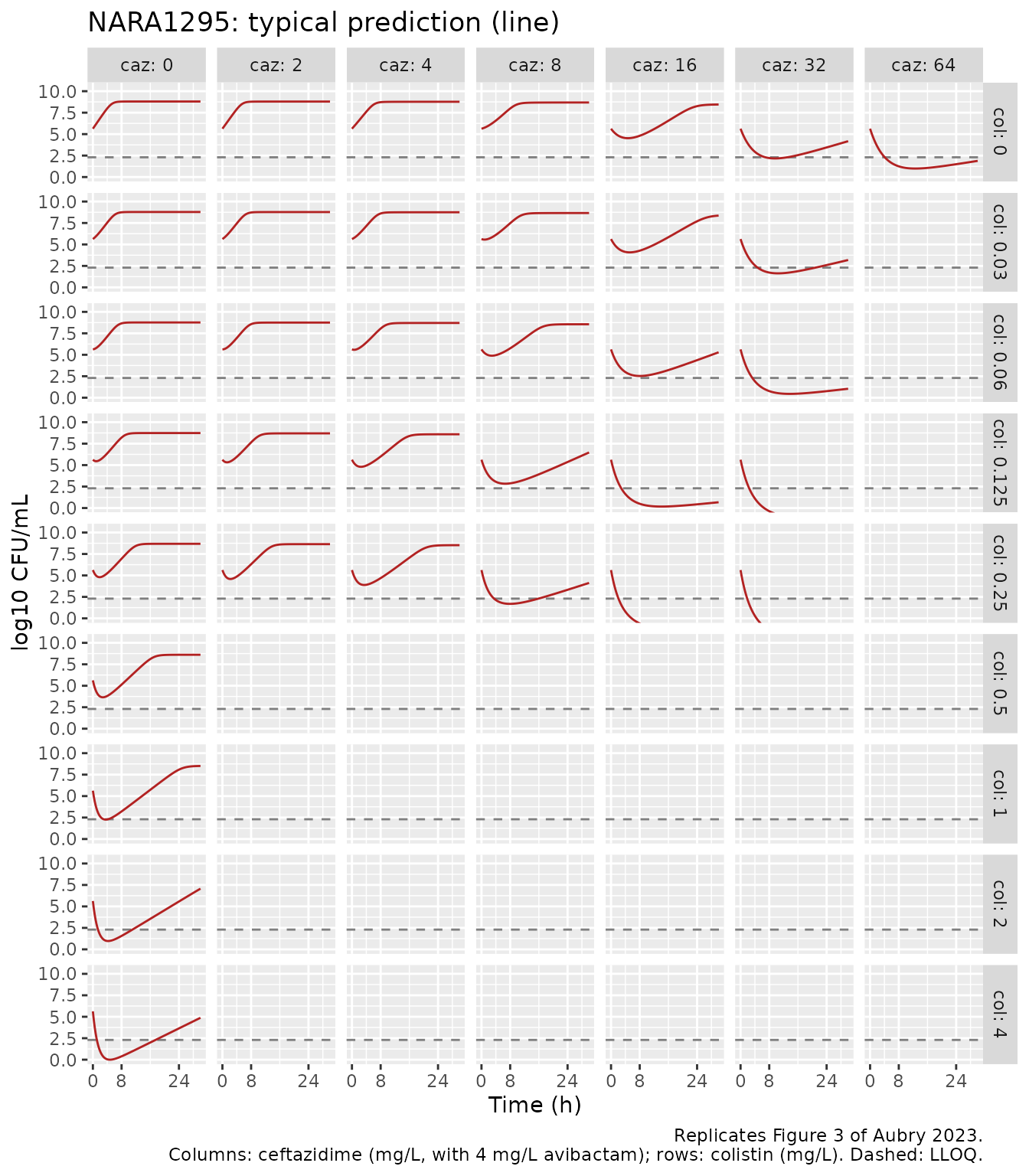
plot_isolate("NARA1584", "Figure S1")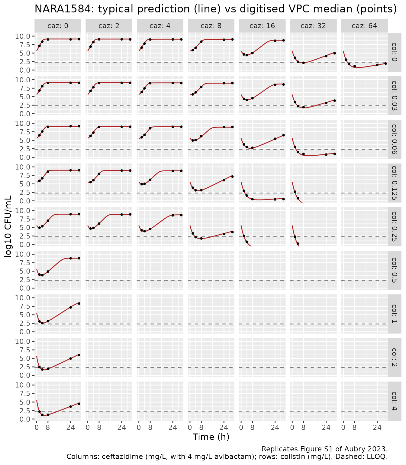
plot_isolate("NARA1182", "Figure S2")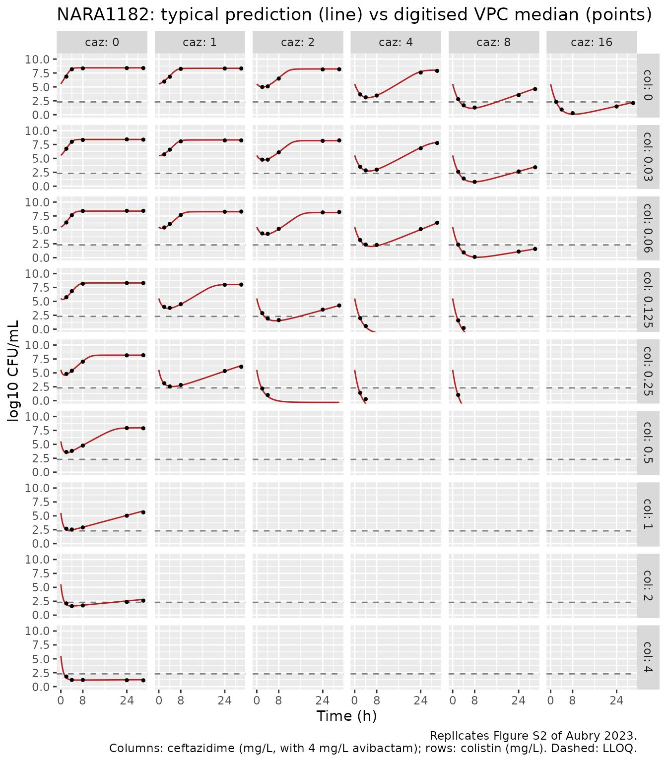
plot_isolate("NARA864", "Figure S3")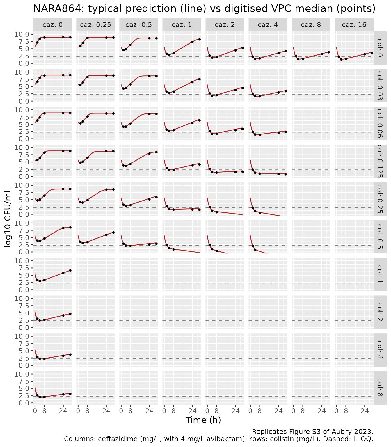
Quantitative agreement
Below the limit of quantification the paper’s plotted medians are clipped at the 0.0 axis line, so the comparison is restricted to points where both the digitised median and the model are above 2.5 log10 CFU/mL.
vpc_cmp <- typ |>
  select(isolate, caz, col, time, log_cfu) |>
  inner_join(dig_long, by = c("isolate", "caz", "col", "time")) |>
  filter(log_cfu_paper > 2.5, log_cfu > 2.5) |>
  mutate(diff = log_cfu - log_cfu_paper)
vpc_sum <- vpc_cmp |>
  group_by(isolate) |>
  summarise(
    n = n(),
    median_diff = median(diff),
    median_abs_diff = median(abs(diff)),
    q90_abs_diff = unname(quantile(abs(diff), 0.9)),
    max_abs_diff = max(abs(diff)),
    .groups = "drop"
  )
knitr::kable(vpc_sum, digits = 3)| isolate | n | median_diff | median_abs_diff | q90_abs_diff | max_abs_diff |
|---|---|---|---|---|---|
| NARA1182 | 97 | 0.014 | 0.051 | 0.137 | 0.238 |
| NARA1584 | 136 | 0.028 | 0.050 | 0.141 | 0.316 |
| NARA864 | 140 | 0.068 | 0.080 | 0.203 | 0.421 |
Residual error: variance, not standard deviation
Table 2 prints RES_ADD as an “additive residual error
(log10CFU/mL)”. The control streams (Codes S1-S2) estimate it as
$SIGMA and use W = SQRT(SIGMA(1)) as the
standard deviation, which means NONMEM reports a variance. The VPC bands
settle the reading. In the growth-control panel the band is the
10th-90th percentile of an additive normal error around a flat median,
so its width is 2 * qnorm(0.9) * SD. Measured on the image
pixels of the growth-control panels (the outer edge lines of the band,
at the plateau): NARA1182 (Fig. S2) 3.14 log10 wide, NARA864 (Fig. S3)
3.81 log10 wide.
res_chk <- data.frame(
  isolate = c("NARA1182", "NARA864"),
  RES_ADD = c(1.44, 2.25),
  band_width_figure = c(3.14, 3.81)
) |>
  mutate(
    sd_from_band = band_width_figure / (2 * qnorm(0.9)),
    sd_if_variance = sqrt(RES_ADD),
    sd_if_sd = RES_ADD,
    addSd_in_file = vapply(isolate, function(i) mods[[i]]$theta[["addSd"]], numeric(1))
  )
knitr::kable(res_chk, digits = 3)| isolate | RES_ADD | band_width_figure | sd_from_band | sd_if_variance | sd_if_sd | addSd_in_file |
|---|---|---|---|---|---|---|
| NARA1182 | 1.44 | 3.14 | 1.225 | 1.2 | 1.44 | 1.2 |
| NARA864 | 2.25 | 3.81 | 1.486 | 1.5 | 2.25 | 1.5 |
stopifnot(
  all(abs(res_chk$sd_from_band - res_chk$sd_if_variance) <
        abs(res_chk$sd_from_band - res_chk$sd_if_sd)),
  all(abs(res_chk$addSd_in_file - res_chk$sd_if_variance) < 1e-8)
)
The variance reading reproduces the band width of both isolates within the pixel resolution; the standard-deviation reading would make the NARA864 band 5.8 log10 wide, half as wide again as printed.
Results-text checks
The Results section reports that each drug alone at its MIC let the bacteria regrow, and that the combination at 2x the MIC of each drug prevented regrowth for every isolate. With the Table 1 MICs:
mic <- data.frame(
  isolate = isolates,
  mic_caz = c(8, 8, 4, 2),
  mic_cst = c(0.125, 0.125, 0.125, 0.25)
)
claims <- bind_rows(lapply(seq_len(nrow(mic)), function(k) {
  i <- mic$isolate[k]
  p <- data.frame(
    scenario = c("CZA 1x MIC alone", "CST 1x MIC alone", "CZA 2x + CST 2x MIC"),
    caz = c(1, 0, 2) * mic$mic_caz[k],
    col = c(0, 1, 2) * mic$mic_cst[k]
  )
  solve_typical(mods[[i]], p) |>
    left_join(p, by = c("caz", "col")) |>
    group_by(scenario) |>
    summarise(nadir = min(log_cfu), at_30h = log_cfu[time == 30], .groups = "drop") |>
    mutate(isolate = i, regrowth = at_30h - nadir)
}))
claims |>
  select(isolate, scenario, nadir, at_30h, regrowth) |>
knitr::kable(digits = 2)| isolate | scenario | nadir | at_30h | regrowth |
|---|---|---|---|---|
| NARA1295 | CST 1x MIC alone | 5.45 | 8.73 | 3.28 |
| NARA1295 | CZA 1x MIC alone | 5.63 | 8.69 | 3.06 |
| NARA1295 | CZA 2x + CST 2x MIC | -1.54 | -1.54 | 0.00 |
| NARA1584 | CST 1x MIC alone | 5.57 | 9.03 | 3.45 |
| NARA1584 | CZA 1x MIC alone | 5.62 | 9.00 | 3.38 |
| NARA1584 | CZA 2x + CST 2x MIC | -2.54 | -2.54 | 0.00 |
| NARA1182 | CST 1x MIC alone | 5.33 | 8.31 | 2.98 |
| NARA1182 | CZA 1x MIC alone | 3.06 | 8.02 | 4.96 |
| NARA1182 | CZA 2x + CST 2x MIC | -6.00 | -6.00 | 0.00 |
| NARA864 | CST 1x MIC alone | 4.70 | 8.69 | 4.00 |
| NARA864 | CZA 1x MIC alone | 1.95 | 5.51 | 3.56 |
| NARA864 | CZA 2x + CST 2x MIC | -2.54 | -2.54 | 0.00 |
Direction of the interaction (Figures 4 and 5)
The paper judged synergy and antagonism by comparing bootstrap 95%
CIs of the observed-interaction model with those of a separately fitted
Bliss expected-additivity model (Code S1), whose parameter estimates are
not tabulated. That comparison cannot be reproduced here, but its
direction can: setting int_col_caz = 0 switches the GPDI
term off while keeping every other parameter. For NARA1295 colistin
lowers the CZA EC50, so the combination kills more than additivity
predicts – the paper finds significant synergy late in the experiment
(Fig. 4); the case below uses both drugs at their MIC (CZA 8 mg/L, CST
0.125 mg/L), where the EC50 shift matters most, since well below the CZA
EC50 there is little CZA kill to enhance. For NARA864 colistin lowers
the CZA Emax, so the combination kills less (the paper finds antagonism
at CZA 0.25-0.5 mg/L with CST 0.25-0.5 mg/L, Fig. 5).
dir_case <- function(i, caz, col) {
  p <- data.frame(caz = caz, col = col)
  obs <- solve_typical(mods[[i]], p, times = c(0, 8, 24, 30))
  add <- solve_typical(rxode2::ini(mods[[i]], int_col_caz = 0), p, times = c(0, 8, 24, 30))
  data.frame(isolate = i, caz = caz, col = col, time = obs$time,
             observed = obs$log_cfu, no_interaction = add$log_cfu)
}
dir_tab <- bind_rows(
  dir_case("NARA1295", 8, 0.125),
  dir_case("NARA864", 0.5, 0.5)
) |>
  mutate(difference = observed - no_interaction)
#> ℹ change initial estimate of `int_col_caz` to `0`
#> ℹ change initial estimate of `int_col_caz` to `0`
knitr::kable(dir_tab, digits = 2)| isolate | caz | col | time | observed | no_interaction | difference |
|---|---|---|---|---|---|---|
| NARA1295 | 8.0 | 0.12 | 0 | 5.63 | 5.63 | 0.00 |
| NARA1295 | 8.0 | 0.12 | 8 | 2.88 | 6.10 | -3.22 |
| NARA1295 | 8.0 | 0.12 | 24 | 5.36 | 8.60 | -3.24 |
| NARA1295 | 8.0 | 0.12 | 30 | 6.47 | 8.60 | -2.13 |
| NARA864 | 0.5 | 0.50 | 0 | 5.68 | 5.68 | 0.00 |
| NARA864 | 0.5 | 0.50 | 8 | 2.22 | 0.78 | 1.44 |
| NARA864 | 0.5 | 0.50 | 24 | 2.90 | -0.44 | 3.35 |
| NARA864 | 0.5 | 0.50 | 30 | 3.17 | -0.90 | 4.06 |
Clinical-profile simulations (Figure 6)
Figure 6 and Figs. S6-S7 drive the NARA1295 model with typical
patient concentration-time profiles from two external popPK models
(ceftazidime from Sy et al. 2019, colistin from Kristoffersson et
al. 2020) that are not in this library, so they are not reproduced here.
The model accepts time-varying CONC_CAZ_MGL /
CONC_CST_MGL columns for that purpose: rxode2 interpolates
covariates between records, and the adaptation switch follows the
instantaneous concentration exactly as IF(A(1).GT.0) does
in Code S2. Note that avibactam is assumed throughout to be present at a
fully inhibiting, non-bactericidal concentration, which the paper flags
as an assumption for these simulations (Discussion).
Assumptions and deviations
-
Residual error is a variance. Table 2
RES_ADDis the NONMEM$SIGMAvariance (see the residual section); each file carriesaddSd = sqrt(RES_ADD). The paper fitted below-quantification counts with Beal’s M3 method (LLOQ 200 CFU/mL); the model files carry the plain additive error, and a user re-estimating with censored data should setCENS/LIMITaccordingly. -
Linear CFU state. Eq 5 calls
Ba log10 count, but the control streams integrateDADT(3) = (KG*PLATEAU - E_COMB)*A(3)withA_0(3) = 10**INOCandPLATEAU = 1 - A(3)/10**BMAX, i.e. logistic growth of the linear CFU/mL count. The files follow the control streams. - Template control stream. Only the NARA1295 control streams are published. The paper states that the same structure was used for all four isolates with isolate-specific estimates, so the other three files reuse the Code S2 structure with their Table 2 column.
-
NARA864 Emax interaction. No control stream is
printed for an interaction on Emax. The file multiplies the CZA Emax by
the GPDI factor
(1 + INT * C_CST / (0.39 + C_CST))and, as in Code S2, keeps the Bliss normaliser at the larger of the two mono-drug Emax values (9.17 1/h). The alternative of normalising by the interaction-reduced Emax was also checked against the digitised Fig. S3 medians and fits marginally worse (90th percentile absolute difference 0.30 versus 0.29 log10). -
Avibactam has no covariate. Every experiment used 4
mg/L, which the authors assume fully inhibits the beta-lactamases with
no bactericidal effect of its own;
CONC_CAZ_MGLis the ceftazidime concentration in the presence of that avibactam. - Interaction gating. Code S2 sets the interaction to zero unless both drugs are present. The files compute it whenever colistin is present; without ceftazidime the ceftazidime kill term is zero, so the two are identical.
-
Observation floor.
log_cfuuses the1e-6CFU/mL floor of the control-stream error block; deep-kill predictions below about -6 log10 are reported as -6. -
Adaptive-resistance state names.
aron_col/aroff_coluse the registered colistin suffix;aron_caz/aroff_cazare declared as paper-specific compartments becausecazis not a registered suffix token.