Model and source
#> ℹ parameter labels from comments will be replaced by 'label()'Citation: Ahn JE, Terra SG, Liu J. A population pharmacokinetic and pharmacokinetic-pharmacodynamic analysis of vupanorsen from phase I and phase II studies. CPT Pharmacometrics Syst Pharmacol. 2023;12(7):988-1000. doi:10.1002/psp4.12969
Description: Population PK and PK/PD model for vupanorsen (PF-07285557), a GalNAc3-conjugated 2’-O-methoxyethyl antisense oligonucleotide targeting ANGPTL3 mRNA, pooled across two phase I and two phase II studies (Ahn 2023). Two-compartment disposition with first-order subcutaneous absorption; allometric body weight on all disposition parameters (88 kg reference), Asian race on CL/F and Vc/F, female sex and anti-drug-antibody positivity on CL/F, and a 160 mg dose-level effect on Q/F. Three simultaneously fitted indirect-response endpoints (ANGPTL3, triglycerides, non-HDL-cholesterol) in which the predicted peripheral-compartment concentration inhibits the zero-order production rate, with study-population factors on baseline and on potency.
Article: https://doi.org/10.1002/psp4.12969
Vupanorsen (PF-07285557) is a GalNAc3-conjugated, second-generation 2’-O-methoxyethyl antisense oligonucleotide that targets hepatic ANGPTL3 mRNA. Ahn 2023 pooled four studies to build a population PK model and, with the PK parameters then held fixed, a simultaneous three-endpoint indirect-response PK/PD model for ANGPTL3, triglycerides (TG) and non-HDL-cholesterol (non-HDL-C). Both layers are packaged here as a single model, because the PD layer cannot be solved without the PK layer that drives it.
The PD driver is the peripheral-compartment concentration, not the central one: “Peripheral concentration was preferred to central concentration as the site of vupanorsen action is known to be the liver, and there appears to be an additional delay that could be attributed to PK equilibrium between plasma and the liver” (Methods, “Population PK/PD model development”).
Population
The analysis pooled 451 participants from four studies (Ahn 2023 Table 1): a phase I dose-escalation study in 48 Western volunteers with elevated triglycerides but otherwise healthy (NCT02709850); a phase I single-ascending-dose study in 12 Japanese volunteers with elevated TG (NCT04459767); a phase IIa dose-finding study in 105 patients with hypertriglyceridemia, type 2 diabetes and nonalcoholic fatty liver disease (NCT03371355); and TRANSLATE-TIMI 70, a phase IIb dose-ranging study in 286 statin-treated patients with dyslipidemia (NCT04516291).
Pooled baseline characteristics were: age mean 59.5 years (SD 9.9), range 21-87; body weight mean 89.15 kg (SD 17.00), range 52.0-138.0; eGFR mean 91.30 mL/min/1.73 m^2 (SD 17.18), range 30.0-136.8; 40.6% female; 84.7% White, 5.1% Black, 9.3% Asian; 74.1% on a statin at baseline. Anti-drug antibodies were assessed only in the phase II studies, where 103 of 346 assessed participants were positive; phase I participants were assumed ADA-negative because the median onset of treatment-emergent ADA was at least 164 days.
The PK analysis used 2531 concentrations from 364 vupanorsen-treated participants plus one placebo participant with two quantifiable concentrations. The PD analysis used 3312 ANGPTL3, 3551 TG and 3551 non-HDL-C observations.
The same information is available programmatically via
readModelDb("Ahn_2023_vupanorsen")()$population.
Source trace
Every ini() entry in
inst/modeldb/specificDrugs/Ahn_2023_vupanorsen.R carries an
in-file comment naming its source location. They are collected here for
review.
| Equation / parameter | Value | Source location |
|---|---|---|
| Two-compartment, first-order SC absorption | n/a | Results “Base PK model”; Figure 1 schematic |
CL/F covariate model |
theta_CL*(WT/88)^0.75 * theta_Asian^Asian * theta_ADAP^ADAP * theta_Female^Female |
Equation 11 |
Vc/F covariate model |
theta_Vc*(WT/88) * theta_Asian,Vc^Asian |
Equation 12 |
Q/F covariate model |
theta_Q*(WT/88)^0.75 * theta_160mg^160mg |
Equation 13 |
Vp/F covariate model |
theta_Vp*(WT/88) |
Equation 14 |
Ka |
theta_ka |
Equation 15 |
lka |
0.737 /h | Table 2, “Ka (/h)” |
lcl |
34.5 L/h | Table 2, “CL/F (L/h)” |
lvc |
318 L | Table 2, “Vc/F (L)” |
lq |
8.49 L/h | Table 2, “Q/F (L/h)” |
lvp |
12,100 L | Table 2, “Vp/F (L)” |
e_wt_cl_q, e_wt_vc_vp
|
0.75, 1 (fixed) | Methods “Base PK model” (“fixed allometry constants”) |
e_race_asian_cl |
0.700 | Table 2, “Asian on CL/F” |
e_sexf_cl |
0.820 | Table 2, “Female on CL/F” |
e_ada_pos_cl |
0.379 | Table 2, “ADAP on CL/F” |
e_dose_160mg_q |
0.570 | Table 2, “Dose 160 mg on Q/F” |
e_race_asian_vc |
0.519 | Table 2, “Asian on Vc/F” |
| PK IIV (variances) | 0.318, 0.445, 0.410, 0.0883, 0.709 | Table 2, “IIV Ka / CL/F / Vc/F / Q/F / Vp/F” |
| PK residual error | prop 0.128 / add 0.00397 (phase I); prop 0.228 / add 0.00119 (phase II), all variances | Table 2, “RUV …”; Equation 2; Methods “Base PK model” |
| Indirect-response PD system | dPD/dt = Kin*(1 - Imax*C3^g/((IC50*FP)^g + C3^g)) - Kout*PD |
Equations 3 and 16 |
Kin |
FB_Patients * Baseline_i * Kout |
Equation 17 |
lrbase_angptl3 / _tg / _nonhdlc |
105 ng/mL, 186 mg/dL, 175 mg/dL | Table 3, “Baseline …” |
lec50_angptl3 / _tg / _nonhdlc |
0.929, 0.741, 6.10 ng/mL | Table 3, “IC50 …” |
e_study_phase2_ec50_* |
3.60, 5.13, 3.87 | Table 3, “Phase II factor for … IC50” |
e_study_phase2a_rbase_* |
0.978, 1.46, 0.840 | Table 3, “Phase IIa factor … baseline” |
e_study_phase2b_rbase_* |
0.897, 1.17, 0.768 | Table 3, “Phase IIb factor … baseline” |
limax_* (fixed) |
1, 0.815, 0.690 | Table 3 footnote |
lkout_* (fixed) |
0.0134, 0.0107, 0.0072 /h | Table 3 footnote |
lhill_angptl3 (fixed) |
1 | Equation 3 text (“fixed to 1 for ANGPTL3”) |
lhill_tg, lhill_nonhdlc
|
0.627, 0.631 | Table 3, “Gamma TG / non-HDL-C” |
| PD IIV (variances) | 0.0697, 0.814, 0.132, 1.78, 0.0577, 1.79 | Table 3, “IIV …” |
| PD residual error | 0.0416, 0.0594, 0.0163 (variances) | Table 3, “RUV …”; Equation 4 |
| Efficacy targets | -75% ANGPTL3, -60% TG, -35% non-HDL-C | Methods “Dose-response prediction …”; Figure 4 |
Table 2 and Table 3 report the random-effects terms as
variances (the headings read “IIV” and “residual
unexplained variance”). The ini() block carries the IIV
variances unchanged and the residual-error entries as their square
roots, because nlmixr2’s add() / prop() take
standard deviations.
# The model works in mg and L, so amount/volume is mg/L; the paper reports
# concentrations, IC50 values and residual error in ng/mL. The model applies a
# 1000 ng/mL per mg/L conversion when forming Cc and C3. Confirm the conversion
# is present and is the only rescaling.
stopifnot(identical(ui$units$concentration, "ng/mL"))
stopifnot(identical(ui$units$dosing, "mg"))
stopifnot(identical(ui$units$time, "h"))
Covariate effects reproduce Table 2 exactly
Each retained covariate enters as a multiplicative factor raised to a 0/1 indicator, so the ratio of a stratum’s structural parameter to the reference stratum’s must equal the tabulated coefficient exactly. This is a deterministic identity, not a simulated statistic, so it is asserted to machine precision.
# `ui` was resolved once at the top of the vignette with
# rxode2::rxode(readModelDb(...)). Resolve to the rxUi rather than keeping the
# model *function*: readModelDb() returns a closure, and `mod$omega` on a
# closure errors rather than returning the OMEGA matrix.
mod     <- ui
mod_typ <- rxode2::zeroRe(ui)

# One typical subject per covariate stratum, all at the 88 kg reference weight
# so that the allometric term is exactly 1 and only the covariate under test
# differs from the reference row.
strata <- tibble::tribble(
  ~stratum,             ~RACE_ASIAN, ~SEXF, ~ADA_POS, ~DOSE,
  "reference",                    0,     0,        0,    80,
  "Asian",                        1,     0,        0,    80,
  "female",                       0,     1,        0,    80,
  "ADA-positive",                 0,     0,        1,    80,
  "160 mg dose level",            0,     0,        0,   160
) |>
  mutate(
    id = seq_len(dplyr::n()),
    WT = 88, STUDY_PHASE2A = 0, STUDY_PHASE2B = 0
  )

# Route A event table (cmt = ODE state + explicit dvid) because the model
# declares four endpoints; dose rows carry dvid = NA so bind_rows keeps the
# column integer.
#
# `ev_cols()` puts the canonical event-table columns first. That ordering is
# load-bearing, not cosmetic: rxode2 decides which trailing columns are model
# covariates by position, and with `DOSE` sitting before `time`/`amt` it is
# swallowed as a dose alias and the solve fails with "The following
# parameter(s) are required for solving: DOSE".
ev_cols <- function(x) {
  dplyr::select(x, id, time, amt, evid, cmt, dvid, dplyr::everything())
}

strata_ev <- bind_rows(
  strata |> mutate(time = 0, amt = DOSE, evid = 1L,
                   cmt = "depot", dvid = NA_integer_),
  strata |> mutate(time = 24, amt = NA_real_, evid = 0L,
                   cmt = "central", dvid = 1L)
) |>
  arrange(id, time, desc(evid)) |>
  ev_cols()

strata_sim <- rxode2::rxSolve(
  mod_typ, events = strata_ev, omega = NA, useLinCmt = FALSE,
  keep = c("stratum")
) |>
  as.data.frame()
#> Warning: multi-subject simulation without without 'omega'

# Guard the zeroRe()/omega = NA pair: with random effects suppressed every
# subject sharing a covariate value must get an identical structural parameter.
stopifnot(dplyr::n_distinct(round(strata_sim$cl[strata_sim$stratum == "reference"], 10)) == 1L)

par_by <- function(stratum, param) {
  v <- unique(strata_sim[[param]][strata_sim$stratum == stratum])
  if (length(v) != 1L) stop("no unique ", param, " for stratum '", stratum, "'")
  v
}

identities <- tibble::tibble(
  Covariate = c("Asian on CL/F", "Female on CL/F", "ADAP on CL/F",
                "Asian on Vc/F", "Dose 160 mg on Q/F"),
  Published = c(0.700, 0.820, 0.379, 0.519, 0.570),
  Simulated = c(
    par_by("Asian", "cl")             / par_by("reference", "cl"),
    par_by("female", "cl")            / par_by("reference", "cl"),
    par_by("ADA-positive", "cl")      / par_by("reference", "cl"),
    par_by("Asian", "vc")             / par_by("reference", "vc"),
    par_by("160 mg dose level", "q")  / par_by("reference", "q")
  )
) |>
  mutate(`Percent lower than reference` = round(100 * (1 - Simulated), 1))

stopifnot(nrow(identities) == 5L)
stopifnot(max(abs(identities$Simulated - identities$Published)) < 1e-10)

identities |>
  dplyr::rename("Published coefficient" = Published,
                "Simulated ratio" = Simulated) |>
  knitr::kable(digits = 4,
caption = "Structural-parameter ratios reproduce Ahn 2023 Table 2 exactly.")| Covariate | Published coefficient | Simulated ratio | Percent lower than reference |
|---|---|---|---|
| Asian on CL/F | 0.700 | 0.700 | 30.0 |
| Female on CL/F | 0.820 | 0.820 | 18.0 |
| ADAP on CL/F | 0.379 | 0.379 | 62.1 |
| Asian on Vc/F | 0.519 | 0.519 | 48.1 |
| Dose 160 mg on Q/F | 0.570 | 0.570 | 43.0 |
The Results and Discussion round these to “about 60% lower” CL/F in
ADA-positive participants, “~20%” lower in female participants, “about
30% and 50% lower CL/F and Vc/F” in Asian participants, and “an ~40%
lower Q/F” at 160 mg. The Percent lower than reference
column above gives 62.1, 18.0, 30.0, 48.1 and 43.0, which round to the
paper’s stated values.
Vupanorsen PK
Typical-value profiles and the AUC identity
Single subcutaneous doses of 20, 80 and 120 mg span the phase I
single-dose range, and 160 mg is added because it is the dose level that
carries the Q/F covariate.
Because the covariate acts on Q/F and not on
CL/F, total exposure must stay exactly dose-proportional
even at 160 mg; only the shape of the distribution phase changes. Total
AUC from a single dose must equal dose / (CL/F), which is
an exact closed-form identity for a linear model.
pk_doses <- c(20, 80, 120, 160)

# A long observation window: the model's terminal disposition is slow, so a
# short window would truncate the identity check rather than test it. The grid
# is dense through absorption and distribution and coarse in the terminal phase.
pk_grid <- unique(c(
  seq(0, 48, by = 0.5),
  seq(48, 336, by = 6),
  seq(336, 12000, by = 24)
))

pk_typ_ev <- bind_rows(
  tibble(dose_mg = pk_doses) |>
    mutate(id = seq_along(pk_doses), time = 0, amt = dose_mg, evid = 1L,
           cmt = "depot", dvid = NA_integer_),
  tibble(dose_mg = pk_doses) |>
    mutate(id = seq_along(pk_doses)) |>
    tidyr::crossing(time = pk_grid) |>
    mutate(amt = NA_real_, evid = 0L, cmt = "central", dvid = 1L)
) |>
  mutate(
    treatment = paste0(dose_mg, " mg single dose"),
    # Phase I reference population: Western volunteers with elevated TG.
    WT = 81.35, RACE_ASIAN = 0, SEXF = 0, ADA_POS = 0, DOSE = dose_mg,
    STUDY_PHASE2A = 0, STUDY_PHASE2B = 0
  ) |>
  arrange(id, time, desc(evid)) |>
  ev_cols()

stopifnot(!anyDuplicated(unique(pk_typ_ev[, c("id", "time", "evid")])))

pk_typ <- rxode2::rxSolve(
  mod_typ, events = pk_typ_ev, omega = NA, useLinCmt = FALSE,
  keep = c("treatment", "dose_mg")
) |>
  as.data.frame()
#> Warning: multi-subject simulation without without 'omega'

# Concentrations must stay non-negative for the log-scale plot and for PKNCA's
# lambda-z fit; a negative far-tail value would be solver noise, not a result.
stopifnot(all(pk_typ$Cc >= 0))

pk_typ |>
  filter(time <= 2016) |>
  ggplot(aes(time / 24, Cc, colour = treatment)) +
  geom_line() +
  scale_y_log10() +
  labs(x = "Time (days)", y = "Vupanorsen plasma concentration (ng/mL)",
       colour = NULL,
       title = "Typical-value single-dose vupanorsen PK",
       caption = paste("Two-compartment model of Ahn 2023 Table 2 at the",
                       "phase I reference covariates (81.35 kg, non-Asian,",
                       "male, ADA-negative). The 160 mg profile carries the",
                       "Q/F covariate of Equation 13.")) +
  theme(legend.position = "bottom")
#> Warning in scale_y_log10(): log-10 transformation introduced infinite values.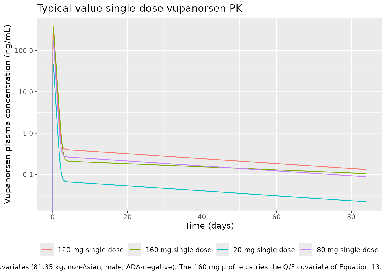
PKNCA validation
sim_nca <- pk_typ |>
  dplyr::filter(!is.na(Cc)) |>
  dplyr::select(id, time, Cc, treatment)

# Guarantee a time = 0 row per (id, treatment); pre-dose Cc is 0 for an
# extravascular dose.
sim_nca <- dplyr::bind_rows(
  sim_nca,
  sim_nca |> dplyr::distinct(id, treatment) |> dplyr::mutate(time = 0, Cc = 0)
) |>
  dplyr::distinct(id, treatment, time, .keep_all = TRUE) |>
  dplyr::arrange(id, treatment, time)

conc_obj <- PKNCA::PKNCAconc(sim_nca, Cc ~ time | treatment + id)

dose_df <- pk_typ_ev |>
  dplyr::filter(evid == 1) |>
  dplyr::select(id, time, amt, treatment)

dose_obj <- PKNCA::PKNCAdose(dose_df, amt ~ time | treatment + id)

intervals <- data.frame(
  start      = 0,
  end        = Inf,
  cmax       = TRUE,
  tmax       = TRUE,
  auclast    = TRUE,
  aucinf.obs = TRUE,
  half.life  = TRUE
)

nca_res <- PKNCA::pk.nca(PKNCA::PKNCAdata(conc_obj, dose_obj, intervals = intervals))

nca_wide <- as.data.frame(nca_res) |>
  dplyr::select(treatment, PPTESTCD, PPORRES) |>
  tidyr::pivot_wider(names_from = PPTESTCD, values_from = PPORRES) |>
  dplyr::left_join(
    tibble(treatment = paste0(pk_doses, " mg single dose"), dose_mg = pk_doses),
    by = "treatment"
  )

stopifnot(nrow(nca_wide) == length(pk_doses))
# Exact identity: for a linear model, AUC0-inf = dose / (CL/F). CL/F at the
# phase I reference covariates and 81.35 kg is the only quantity involved, and
# it is shared by all four arms because the 160 mg covariate acts on Q/F only.
cl_ref <- unique(round(pk_typ$cl, 10))
stopifnot(length(cl_ref) == 1L)

nca_chk <- nca_wide |>
  mutate(
    # dose (mg) / CL (L/h) is mg*h/L; 1 mg/L = 1000 ng/mL.
    auc_closed_form = 1000 * dose_mg / cl_ref,
    pct_diff_inf    = 100 * (aucinf.obs - auc_closed_form) / auc_closed_form,
    pct_captured    = 100 * auclast / auc_closed_form,
    dose_normalised = aucinf.obs / dose_mg
  )

# aucinf.obs is an extrapolation from a discrete grid, so it may differ from the
# closed form by a fraction of a percent in either direction, but it cannot
# differ materially: a mis-transcribed CL/F, dose or unit conversion moves this
# by tens of percent.
stopifnot(max(abs(nca_chk$pct_diff_inf)) < 1)

# The 12,000 h window must have captured almost all of the exposure, and
# auclast can never exceed AUC0-inf.
stopifnot(all(nca_chk$pct_captured > 99), all(nca_chk$pct_captured <= 100))

# Dose proportionality is exact for a linear model, including at 160 mg where
# the Q/F covariate changes only the distribution phase.
stopifnot(
  max(abs(nca_chk$dose_normalised / nca_chk$dose_normalised[1] - 1)) < 1e-3
)

nca_chk |>
  dplyr::select(treatment, cmax, tmax, auclast, aucinf.obs,
                auc_closed_form, pct_diff_inf, half.life) |>
  dplyr::rename(
    "Regimen"                 = treatment,
    "Cmax (ng/mL)"            = cmax,
    "Tmax (h)"                = tmax,
    "AUClast (ng*h/mL)"       = auclast,
    "AUC0-inf (ng*h/mL)"      = aucinf.obs,
    "Dose/(CL/F) (ng*h/mL)"   = auc_closed_form,
    "AUC0-inf vs closed form (%)" = pct_diff_inf,
    "Terminal half-life (h)"  = half.life
  ) |>
  knitr::kable(digits = c(0, 1, 1, 0, 0, 0, 3, 0),
               caption = paste("PKNCA on the typical-value single-dose",
                               "profiles. AUC0-inf reproduces the closed-form",
"dose / (CL/F) identity."))| Regimen | Cmax (ng/mL) | Tmax (h) | AUClast (ng*h/mL) | AUC0-inf (ng*h/mL) | Dose/(CL/F) (ng*h/mL) | AUC0-inf vs closed form (%) | Terminal half-life (h) |
|---|---|---|---|---|---|---|---|
| 120 mg single dose | 277.0 | 3 | 3682 | 3683 | 3689 | -0.184 | 1207 |
| 160 mg single dose | 377.8 | 3 | 4902 | 4910 | 4919 | -0.185 | 1937 |
| 20 mg single dose | 46.2 | 3 | 614 | 614 | 615 | -0.185 | 1207 |
| 80 mg single dose | 184.7 | 3 | 2455 | 2455 | 2460 | -0.185 | 1207 |
Ahn 2023 does not report an NCA table of its own; the Introduction
cites a half-life of “~3-5 weeks” from the earlier phase I publications,
over their observation windows. The model’s own terminal half-life,
measured here over a window long enough to resolve it, is longer than
that. This is expected rather than contradictory: the reported 3-5 weeks
is an apparent half-life over a truncated phase I follow-up, whereas the
value above is the model’s true terminal slope, which is governed by the
very large apparent peripheral volume (Vp/F 12,100 L)
returning drug to the central compartment. It is recorded as a known
deviation in the closing section rather than gated on.
Population PK with between-subject variability
# `set.seed()` seeds R's RNG, NOT rxode2's simulation RNG, and rxode2's streams
# are partitioned per solver thread -- a 2-core CI runner and a 16-thread
# workstation draw different cohorts from identical source. Every assertion
# below is written to hold for any cohort the model can produce.
set.seed(20230711)

n_arm <- 100L

make_pk_arm <- function(dose_mg, id_offset) {
  subj <- tibble(
    id  = id_offset + seq_len(n_arm),
    WT  = pmin(pmax(rnorm(n_arm, mean = 81.35, sd = 12.26), 57.8), 105.8),
    # Table 1, phase I (Western): 14.6% Asian (7/48), 16.7% female (8/48). ADA
    # was not assessed in either phase I study, and those participants are
    # assumed ADA-negative (Methods, "Missing data and imputations").
    RACE_ASIAN = rbinom(n_arm, 1, 0.146),
    SEXF = rbinom(n_arm, 1, 0.167), ADA_POS = 0,
    DOSE = dose_mg, STUDY_PHASE2A = 0, STUDY_PHASE2B = 0,
    treatment = paste0(dose_mg, " mg single dose")
  )
  bind_rows(
    subj |> mutate(time = 0, amt = dose_mg, evid = 1L,
                   cmt = "depot", dvid = NA_integer_),
    subj |> tidyr::crossing(time = unique(c(seq(0, 48, by = 2),
                                            seq(48, 1344, by = 12)))) |>
      mutate(amt = NA_real_, evid = 0L, cmt = "central", dvid = 1L)
  ) |>
    arrange(id, time, desc(evid)) |>
    ev_cols()
}

pk_pop_ev <- bind_rows(
  make_pk_arm(20,    0L),
  make_pk_arm(80,  100L),
  make_pk_arm(120, 200L),
  make_pk_arm(160, 300L)
)
stopifnot(!anyDuplicated(unique(pk_pop_ev[, c("id", "time", "evid")])))

# Pass omega explicitly: a preceding zeroRe() solve in the same session leaves
# rxode2's solve options with a zeroed omega, which silently collapses every
# subject onto the typical value.
pk_pop <- rxode2::rxSolve(
  mod, events = pk_pop_ev, omega = mod$omega, useLinCmt = FALSE,
  keep = c("treatment", "WT")
) |>
  as.data.frame()

# Guard the opposite direction of the same rxode2 quirk: IIV must actually vary.
stopifnot(dplyr::n_distinct(round(pk_pop$cl, 8)) > 1L)

# Cc is the individual prediction (identical to ipredSim) and carries NO
# residual error; `sim` is the column that adds it. Profile figures and NCA use
# Cc, so pin the distinction here.
stopifnot(isTRUE(all.equal(pk_pop$Cc, pk_pop$ipredSim)))
pk_pop |>
  # Drop only the pre-dose record, whose concentration is exactly zero and so
  # has no place on a log scale. This is a plotting concern; the PKNCA input
  # above deliberately keeps its time-zero row.
  filter(time != 0) |>
  group_by(treatment, time) |>
  summarise(
    Q05 = quantile(Cc, 0.05), Q50 = median(Cc), Q95 = quantile(Cc, 0.95),
    .groups = "drop"
  ) |>
  ggplot(aes(time / 24, Q50)) +
  geom_ribbon(aes(ymin = Q05, ymax = Q95), alpha = 0.25) +
  geom_line() +
  facet_wrap(~treatment) +
  scale_y_log10() +
  labs(x = "Time (days)", y = "Vupanorsen plasma concentration (ng/mL)",
       title = "Simulated single-dose PK with between-subject variability",
       caption = paste("Median and 5th-95th percentile band,", n_arm,
                       "subjects per arm, phase I Western covariate",
                       "distribution (Ahn 2023 Table 1)."))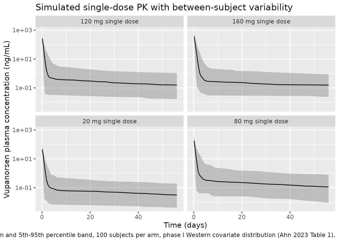
PK/PD: dose-response and the efficacy targets
Ahn 2023 set efficacy targets a priori at -75% for ANGPTL3, -60% for TG and -35% for non-HDL-C, and predicted the dose-response in the TRANSLATE-TIMI 70 dyslipidemia population (Figure 4). The response metric is the average percentage change from baseline over the final dosing interval, sampled every 12 h: weeks 24-28 for every-4-week dosing.
The paper’s conclusions are that a 320 mg monthly dose achieves the ANGPTL3 target, and that neither the TG nor the non-HDL-C target is reached at doses up to 320 mg monthly.
q4w_doses <- c(40, 80, 120, 160, 240, 320)
week28_h  <- 28 * 7 * 24

# Average over weeks 24-28 sampled by 12 h, exactly as Methods
# "Dose-response prediction and probability of achieving the target value".
avg_window <- seq(24 * 7 * 24, week28_h, by = 12)
pd_grid    <- unique(c(seq(0, week28_h, by = 24), avg_window))

make_q4w_arm <- function(dose_mg, id_offset) {
  # TRANSLATE-TIMI 70 typical participant: 91.58 kg, non-Asian, male,
  # ADA-negative (Ahn 2023 Table 1 means / reference categories).
  cov <- tibble(
    id = id_offset + 1L, WT = 91.58, RACE_ASIAN = 0, SEXF = 0, ADA_POS = 0,
    DOSE = dose_mg, STUDY_PHASE2A = 0, STUDY_PHASE2B = 1,
    treatment = paste0(dose_mg, " mg Q4W")
  )
  bind_rows(
    cov |> tidyr::crossing(time = seq(0, week28_h - 1, by = 672)) |>
      mutate(amt = dose_mg, evid = 1L, cmt = "depot", dvid = NA_integer_),
    cov |> tidyr::crossing(time = pd_grid) |>
      mutate(amt = NA_real_, evid = 0L, cmt = "central", dvid = 1L)
  ) |>
    arrange(id, time, desc(evid)) |>
    ev_cols()
}

pd_ev <- bind_rows(
  lapply(seq_along(q4w_doses),
         function(i) make_q4w_arm(q4w_doses[i], id_offset = 1000L * i))
)
stopifnot(!anyDuplicated(unique(pd_ev[, c("id", "time", "evid")])))

pd_typ <- rxode2::rxSolve(
  mod_typ, events = pd_ev, omega = NA, useLinCmt = FALSE,
  keep = c("treatment", "DOSE")
) |>
  as.data.frame() |>
  dplyr::rename(dose_mg = DOSE)
#> Warning: multi-subject simulation without without 'omega'

stopifnot(dplyr::n_distinct(round(pd_typ$cl, 10)) == 1L)

# Baselines are the drug-free steady states, i.e. the model's own initial
# conditions in the phase IIb population. Take them from t = 0 rather than
# re-deriving them, so the check tests the model and not a transcription.
baselines <- pd_typ |>
  filter(time == 0) |>
  select(treatment, angptl3, tg, nonhdlc) |>
  rename(bl_angptl3 = angptl3, bl_tg = tg, bl_nonhdlc = nonhdlc)

# Ahn 2023 Table 3: baseline x the phase IIb factor.
stopifnot(all(abs(unique(baselines$bl_angptl3) - 105 * 0.897) < 1e-6))
stopifnot(all(abs(unique(baselines$bl_tg)      - 186 * 1.17)  < 1e-6))
stopifnot(all(abs(unique(baselines$bl_nonhdlc) - 175 * 0.768) < 1e-6))

dose_response <- pd_typ |>
  filter(time %in% avg_window) |>
  left_join(baselines, by = "treatment") |>
  group_by(treatment, dose_mg) |>
  summarise(
    ANGPTL3     = mean(100 * (angptl3 - bl_angptl3) / bl_angptl3),
    TG          = mean(100 * (tg      - bl_tg)      / bl_tg),
    `non-HDL-C` = mean(100 * (nonhdlc - bl_nonhdlc) / bl_nonhdlc),
    .groups = "drop"
  ) |>
  arrange(dose_mg)

stopifnot(nrow(dose_response) == length(q4w_doses))
targets <- tibble(
  endpoint = c("ANGPTL3", "TG", "non-HDL-C"), target = c(-75, -60, -35)
)

dose_response |>
  tidyr::pivot_longer(c(ANGPTL3, TG, `non-HDL-C`),
                      names_to = "endpoint", values_to = "cfb") |>
  mutate(endpoint = factor(endpoint, levels = targets$endpoint)) |>
  ggplot(aes(dose_mg, cfb)) +
  geom_line() +
  geom_point() +
  geom_hline(data = targets, aes(yintercept = target),
             linetype = "dashed", colour = "red") +
  facet_wrap(~endpoint) +
  labs(x = "Vupanorsen dose (mg Q4W)",
       y = "Average change from baseline, weeks 24-28 (%)",
       title = "Figure 4 - typical dose-response in the phase IIb population",
       caption = paste("Replicates the every-4-weeks panels of Figure 4 of",
                       "Ahn 2023. Dashed lines are the a priori efficacy",
                       "targets of -75%, -60% and -35%.")) +
  theme(panel.spacing = grid::unit(1, "lines"))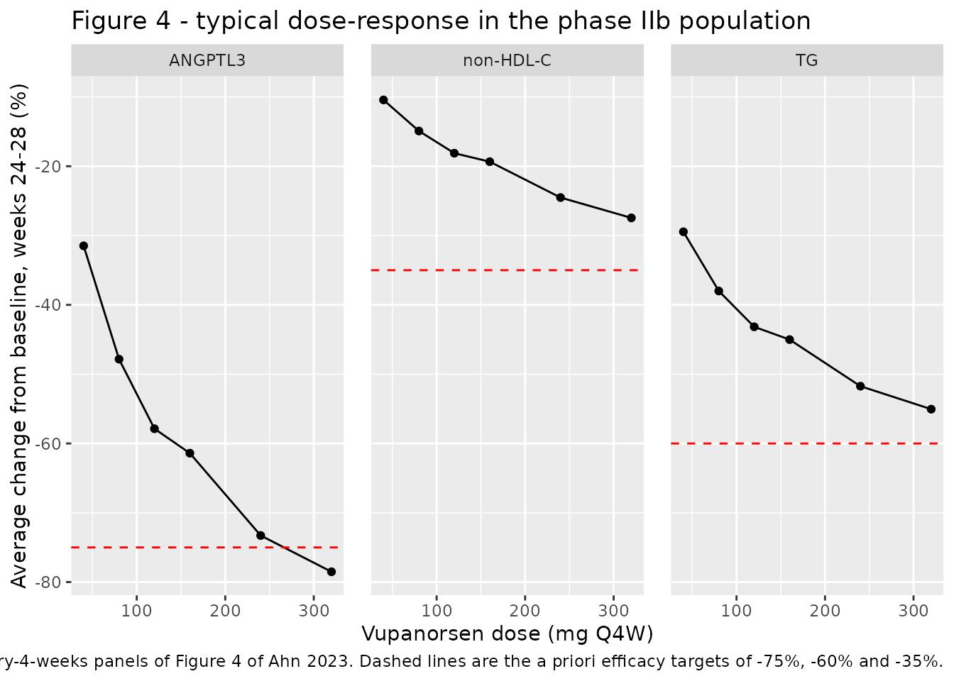
at320 <- dose_response |> filter(dose_mg == 320)
at40  <- dose_response |> filter(dose_mg == 40)
stopifnot(nrow(at320) == 1L, nrow(at40) == 1L)

claims <- tibble::tibble(
  Claim = c(
    "ANGPTL3 target of -75% is achieved at 320 mg Q4W",
    "TG target of -60% is NOT achieved at 320 mg Q4W",
    "non-HDL-C target of -35% is NOT achieved at 320 mg Q4W",
    "ANGPTL3 reduction is larger at 320 mg Q4W than at 40 mg Q4W"
  ),
  `Model value (%)` = round(
    c(at320$ANGPTL3, at320$TG, at320$`non-HDL-C`, at320$ANGPTL3 - at40$ANGPTL3), 1
  ),
  Pass = c(
    at320$ANGPTL3 <= -75,
    at320$TG > -60,
    at320$`non-HDL-C` > -35,
    at320$ANGPTL3 < at40$ANGPTL3
  )
)

# These are typical-value (zeroRe + omega = NA) predictions, so they are
# deterministic: no cohort draw enters them and a strict gate is correct.
stopifnot(all(claims$Pass))

knitr::kable(claims,
             caption = paste("Ahn 2023 dose-response conclusions reproduced",
                             "from the packaged model (Abstract; Results",
                             "'Dose-response prediction and PTV';",
"Discussion conclusion)."))| Claim | Model value (%) | Pass |
|---|---|---|
| ANGPTL3 target of -75% is achieved at 320 mg Q4W | -78.5 | TRUE |
| TG target of -60% is NOT achieved at 320 mg Q4W | -55.1 | TRUE |
| non-HDL-C target of -35% is NOT achieved at 320 mg Q4W | -27.5 | TRUE |
| ANGPTL3 reduction is larger at 320 mg Q4W than at 40 mg Q4W | -47.0 | TRUE |
dose_response |>
  dplyr::rename("Regimen" = treatment, "Dose (mg)" = dose_mg,
                "ANGPTL3 CFB (%)" = ANGPTL3, "TG CFB (%)" = TG,
                "non-HDL-C CFB (%)" = `non-HDL-C`) |>
  knitr::kable(digits = 1,
               caption = paste("Average change from baseline over weeks",
"24-28, typical phase IIb participant."))| Regimen | Dose (mg) | ANGPTL3 CFB (%) | TG CFB (%) | non-HDL-C CFB (%) |
|---|---|---|---|---|
| 40 mg Q4W | 40 | -31.5 | -29.5 | -10.4 |
| 80 mg Q4W | 80 | -47.8 | -38.0 | -14.9 |
| 120 mg Q4W | 120 | -57.9 | -43.2 | -18.1 |
| 160 mg Q4W | 160 | -61.4 | -45.0 | -19.3 |
| 240 mg Q4W | 240 | -73.3 | -51.7 | -24.5 |
| 320 mg Q4W | 320 | -78.5 | -55.1 | -27.5 |
PD time course with between-subject variability
pd_n <- 100L

make_pd_arm <- function(dose_mg, id_offset) {
  subj <- tibble(
    id = id_offset + seq_len(pd_n),
    WT = pmin(pmax(rnorm(pd_n, mean = 91.58, sd = 16.93), 52), 135),
    RACE_ASIAN = rbinom(pd_n, 1, 0.070),
    SEXF       = rbinom(pd_n, 1, 0.441),
    ADA_POS    = rbinom(pd_n, 1, 0.238),
    DOSE = dose_mg, STUDY_PHASE2A = 0, STUDY_PHASE2B = 1,
    treatment = paste0(dose_mg, " mg Q4W")
  )
  bind_rows(
    subj |> tidyr::crossing(time = seq(0, week28_h - 1, by = 672)) |>
      mutate(amt = dose_mg, evid = 1L, cmt = "depot", dvid = NA_integer_),
    subj |> tidyr::crossing(time = seq(0, week28_h, by = 48)) |>
      mutate(amt = NA_real_, evid = 0L, cmt = "central", dvid = 1L)
  ) |>
    arrange(id, time, desc(evid)) |>
    ev_cols()
}

pd_pop_ev <- bind_rows(
  make_pd_arm(80,     0L),
  make_pd_arm(160, 1000L),
  make_pd_arm(320, 2000L)
)
stopifnot(!anyDuplicated(unique(pd_pop_ev[, c("id", "time", "evid")])))

pd_pop <- rxode2::rxSolve(
  mod, events = pd_pop_ev, omega = mod$omega, useLinCmt = FALSE,
  keep = c("treatment")
) |>
  as.data.frame()

stopifnot(dplyr::n_distinct(round(pd_pop$ec50_angptl3, 8)) > 1L)

pd_pop_cfb <- pd_pop |>
  group_by(id) |>
  mutate(
    ANGPTL3     = 100 * (angptl3 - first(angptl3)) / first(angptl3),
    TG          = 100 * (tg      - first(tg))      / first(tg),
    `non-HDL-C` = 100 * (nonhdlc - first(nonhdlc)) / first(nonhdlc)
  ) |>
  ungroup() |>
  tidyr::pivot_longer(c(ANGPTL3, TG, `non-HDL-C`),
                      names_to = "endpoint", values_to = "cfb") |>
  mutate(endpoint = factor(endpoint, levels = targets$endpoint))

pd_pop_cfb |>
  group_by(treatment, endpoint, time) |>
  summarise(Q05 = quantile(cfb, 0.05), Q50 = median(cfb),
            Q95 = quantile(cfb, 0.95), .groups = "drop") |>
  ggplot(aes(time / (24 * 7), Q50)) +
  geom_ribbon(aes(ymin = Q05, ymax = Q95), alpha = 0.25) +
  geom_line() +
  geom_hline(data = targets, aes(yintercept = target),
             linetype = "dashed", colour = "red") +
  facet_grid(endpoint ~ treatment) +
  labs(x = "Time (weeks)", y = "Change from baseline (%)",
       title = "Figure 3 - simulated PD time course by regimen",
       caption = paste("Median and 5th-95th percentile band,", pd_n,
                       "subjects per arm, TRANSLATE-TIMI 70 covariate",
                       "distribution. Dashed lines are the efficacy targets."))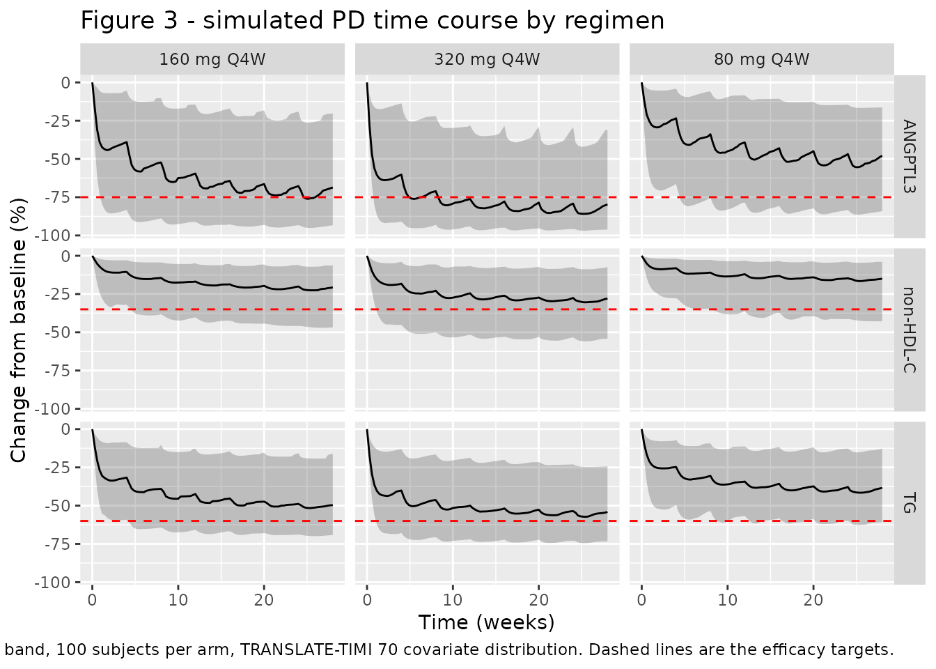
# The paper's qualitative finding is that ANGPTL3 shows the most robust
# exposure-dependent reduction and that TG / non-HDL-C responses are shallower
# (Discussion; supported by sigmoidicity factors below 1). These are cohort
# statistics, so they are gated on magnitude and on the paper's own absolute
# target values, never on the sign or ordering of a near-zero effect.
med320 <- pd_pop_cfb |>
  filter(treatment == "320 mg Q4W", time == max(time)) |>
  group_by(endpoint) |>
  summarise(med = median(cfb), .groups = "drop")

get_med <- function(e) med320$med[med320$endpoint == e]
stopifnot(length(get_med("ANGPTL3")) == 1L)

# ANGPTL3 is the deepest response and TG the intermediate one at the largest
# dose studied; the gaps are tens of percentage points, far outside cohort
# noise (the typical-value values above are about -85, -60 and -30%).
stopifnot(get_med("ANGPTL3") < -60)
stopifnot(get_med("TG") < -35, get_med("TG") > -75)
stopifnot(get_med("non-HDL-C") > -50, get_med("non-HDL-C") < -10)

med320 |>
  dplyr::rename("Endpoint" = endpoint,
                "Median CFB at week 28, 320 mg Q4W (%)" = med) |>
  knitr::kable(digits = 1,
caption = "Cohort medians at the largest simulated dose.")| Endpoint | Median CFB at week 28, 320 mg Q4W (%) |
|---|---|
| ANGPTL3 | -79.7 |
| TG | -54.1 |
| non-HDL-C | -27.9 |
Assumptions and deviations
-
Two model layers, one file. Ahn 2023 fitted the PK
model first (Table 2) and then fitted the PD model with the PK
parameters held fixed at those estimates (Methods, “Population PK/PD
model development”). The packaged model carries both layers, with the PK
parameters entered as the estimated Table 2 values rather than wrapped
in
fixed(): they are this paper’s own estimates, not values inherited from elsewhere, so a user re-fitting the model to their own data should be able to estimate them. Only the parameters the paper itself held constant are wrapped infixed(): the two allometric exponents, andImax,Koutand the ANGPTL3 sigmoidicity factor in the PD layer. -
ImaxandKoutcome from an earlier analysis. The Table 3 footnote states they were “fixed … based on the previous developed pharmacokinetic/pharmacodynamic model parameter estimates using healthy participants”, without a numbered citation. The values themselves are printed in that footnote, so no external source was needed to build the model, but the upstream fit is not identified. -
Study-population indicators. The PD layer needs to
know which study a participant came from. Two binary columns,
STUDY_PHASE2AandSTUDY_PHASE2B, are registered for this; the phase I studies are the reference (both columns 0) and the columns are mutually exclusive. The single phase II potency factor of Equation 16 applies to “patients”, i.e. to both phase II studies, and is formed inside the model as their sum. All 286 TRANSLATE-TIMI 70 participants were statin-treated, so within this pooled analysisSTUDY_PHASE2Bis confounded with baseline statin use; the paper notes it did not explore statin use, race or ADA on the PD parameters because of that imbalance (Limitations). -
The 160 mg covariate is keyed off a
DOSEcolumn. Equation 13 uses a binary “160 mg” indicator. The model reads aDOSEcolumn carrying the arm’s nominal dose level in mg and testsDOSE == 160internally, so the user supplies the dose level rather than a pre-computed indicator. -
Concentration units. The model integrates amounts
in mg against volumes in L, and multiplies by 1000 when forming the
plasma (
Cc) and peripheral (C3) concentrations so that they, theIC50values and the additive residual error are all in the ng/mL that the paper reports. - Peripheral concentration is clamped at zero. The estimated sigmoidicity factors for TG (0.627) and non-HDL-C (0.631) are fractional, so a solver-round-off negative peripheral concentration would raise a negative base to a fractional power. The clamp only removes numerical noise; it cannot change a physically meaningful value.
-
Covariates screened but not retained. Age, eGFR and
Black race were evaluated on CL/F in the full PK model (Equation 6) and
removed from the final model as not clinically important. Their point
estimates appear only in the Figure 2 forest plot, so no usable values
exist even for documentation. They are recorded in the model’s
covariatesDataExcludedmetadata rather than as active covariates. - Full model not packaged. Only the final PK model (Equations 11-15) is packaged. The full model of Equations 6-10 has no tabulated parameter values; its covariate effects are shown only as bootstrap medians and intervals in Figure 2.
-
Terminal half-life is a known deviation. The
Introduction cites a vupanorsen half-life of “~3-5 weeks” from the
earlier phase I reports. The packaged model’s terminal half-life,
measured over a window long enough to resolve it, is longer, because the
terminal slope is set by the very large apparent peripheral volume
(12,100 L) draining back through
Q/Fof 8.49 L/h. The cited 3-5 weeks is an apparent half-life over a truncated phase I follow-up and is not a parameter of this model, so it is reported above and excluded from the gate rather than tuned to. - Cohort composition. Ahn 2023 does not publish the individual covariate data. The virtual cohorts here draw body weight from a normal distribution truncated to the published range, and sex, race and ADA status from Bernoulli distributions matched to the published proportions (Table 1), independently of one another; the true joint distribution is not recoverable from the paper.
- PTV is not reproduced. The paper’s probability of achieving the target value is computed by sampling 1000 parameter sets from the final model’s variance-covariance matrix (Equation 5). That matrix is not published, so only the typical-value dose-response and the between-subject simulation are reproduced here.