Mycophenolic acid (Barau 2012)
Source:vignettes/articles/Barau_2012_mycophenolic_acid.Rmd
Barau_2012_mycophenolic_acid.RmdModel and source
- Citation: Barau C, Furlan V, Debray D, Taburet AM, Barrail-Tran A. Population pharmacokinetics of mycophenolic acid and dose optimization with limited sampling strategy in liver transplant children. Br J Clin Pharmacol. 2012;74(3):515-524. doi:10.1111/j.1365-2125.2012.04213.x
- Description: One-compartment population PK model for mycophenolic acid (MPA, active moiety of mycophenolate mofetil MMF) after oral MMF dosing in paediatric liver transplant recipients (Barau 2012). First-order absorption and first-order elimination, with diagonal (uncorrelated) inter-individual variability on ka, CL/F, and V/F and proportional residual error. Two covariates are retained in the final model: a linear-with-age effect on ka of the form ka_TV = 3.9 - 2.2 * (AGE / 8.65 years), so ka declines from 3.9 1/h at AGE = 0 to 1.7 1/h at the cohort median age of 8.65 years; and a power-on-binary effect on V/F of the form V/F = 64.7 L * 2.3^POSTTX_EARLY, where POSTTX_EARLY = 1 within the first 6 months post-transplant (POD <= 180 days) and 0 thereafter, so V/F is 64.7 L in the stable post-transplant period and 148.8 L in the immediate post-transplant period (paper attributes the volume increase to the higher unbound MPA fraction associated with low serum albumin in the immediate post-transplant period). Apparent clearance CL/F = 12.7 L/h carries no retained covariate effect in the final model. Enterohepatic recirculation, the MPAG metabolite compartment, and protein binding are not modelled here – the paper attributes the absence of secondary peaks to surgical removal of the gallbladder in the liver-transplant recipients.
- Article: https://doi.org/10.1111/j.1365-2125.2012.04213.x
Population
The model was developed on 16 paediatric liver transplant recipients with intensive pharmacokinetic sampling (predose plus 0.5, 1, 2, 4, 6, 8 hours after the morning mycophenolate mofetil dose, on a single occasion per subject) followed at the Hopitaux Universitaires Paris-Sud in Le Kremlin Bicetre, France between October 2006 and August 2010 (Barau 2012 Methods, “Patients and study design”). Median age was 8.7 years (range 1.1-15.2) and median weight 23.8 kg (range 9.3-49.2) in the model-building set; sex was balanced (14 boys and 14 girls in the full 28-patient cohort, of which 16 were used for model building and 12 for model validation). Indications for liver transplantation were biliary atresia (14 of 28), fulminant hepatitis (8), progressive familial intrahepatic cholestasis (3), and one each of Alagille syndrome, cystic fibrosis, and Wilson disease. Median time since transplantation was 17.2 months (range 0.2-188.5 months); 7 of the 16 model-building patients were in the immediate post-transplant period (<= 6 months, POSTTX_EARLY = 1) and 9 in the stable post-transplant period (> 6 months, POSTTX_EARLY = 0). MMF dosing was 186-594 mg/m^2 twice daily (median 380 mg/m^2 = 13.0 mg/kg) targeting an MPA AUC(0,12h) between 30 and 60 mg/L*h. Co-medication was tacrolimus (n = 23) or ciclosporin (n = 5) plus steroids (n = 14). Cohort serum albumin was median 31.7 g/L (range 17.2-35.0).
The same information is available programmatically via
readModelDb("Barau_2012_mycophenolic_acid")$population.
Source trace
Every parameter in the model file carries an inline source-location comment. The table below collects the entries in one place.
| Equation / parameter | Value | Source location |
|---|---|---|
lka (ka intercept at AGE = 0) |
3.9 1/h | Table 2, Final model column, k_a row |
e_age_ka (slope on AGE / 8.65) |
2.2 | Table 2, Final model column, b_age_ka row |
lcl (CL/F) |
12.7 L/h | Table 2, Final model column, CL/F row |
lvc (V/F in stable post-transplant period) |
64.7 L | Table 2, Final model column, V/F row |
e_posttx_early_vc (V/F fold-change in <= 6 months
period) |
2.3 | Table 2, Final model column, b_time_V/F row |
| IIV ka (omega^2 = log(1 + 3.084^2) = 2.3524) | 308.4% CV | Table 2, Final model column, omega_ka row |
| IIV CL/F (omega^2 = log(1 + 0.284^2) = 0.0776) | 28.4% CV | Table 2, Final model column, omega_CL/F row |
| IIV V/F (omega^2 = log(1 + 0.418^2) = 0.1610) | 41.8% CV | Table 2, Final model column, omega_V/F row |
| Proportional residual error | 59.6% | Table 2, Final model column, sigma row |
| ka covariate equation | – | Results, “Covariate model building” subsection (k_a,i = (k_aTV - b_age_ka * (age_i / 8.65)) * exp(eta_ka)) |
| V/F covariate equation | – | Results, “Covariate model building” subsection (V/F_i = (V/F_TV * b_time_V/F^time_post_transplantation) * exp(eta_V/F)) |
| Time-post-transplantation cutoff at 6 months | – | Results, “Covariate model building” subsection (“when the time post transplantation was 0 if the patient was in the stable post transplantation period and 1 if the patient was in the immediate post transplantation period”) |
| 1-compartment, first-order absorption + elimination | – | Methods, “Population pharmacokinetic modelling of total MPA” |
| Diagonal Omega matrix | – | Methods, “Population pharmacokinetic modelling of total MPA” (“a diagonal variance matrix Omega was chosen”) |
Virtual cohort
The published dataset is not openly available, so the virtual cohort below mirrors the demographics in Barau 2012 Methods + Table 1. Two sub-cohorts are built so the post-transplant-period stratification replicates the paper’s Figure 1 (concentration vs. time, stratified by <= 6 months vs > 6 months).
The AGE distribution is truncated to the model-building cohort’s
observed range (1.1-15.2 years) so the typical-value ka remains positive
across every simulated subject. At AGE = 15.34 years the published
linear-in-age form ka_TV = 3.9 - 2.2 * AGE / 8.65 reaches
zero; subjects above this age have a mathematically negative typical ka
with the linear form (see “Assumptions and deviations” below).
set.seed(20120101)

n_per_arm <- 200L

# Truncated normal sampler on [lo, hi] around (mu, sd).
rtnorm <- function(n, mu, sd, lo, hi) {
  x <- numeric(0)
  while (length(x) < n) {
    new <- rnorm(2 * n, mu, sd)
    new <- new[new >= lo & new <= hi]
    x <- c(x, new)
  }
  x[seq_len(n)]
}

make_cohort <- function(n, pod_days, label, id_offset = 0L) {
  tibble(
    id     = id_offset + seq_len(n),
    AGE    = rtnorm(n, mu = 8.65, sd = 3.5, lo = 1.1, hi = 15.0),
    WT     = pmax(rnorm(n, mean = 23.8, sd = 9.0), 9.3),
    POD    = pod_days,
    cohort = label
  )
}

demo <- bind_rows(
  make_cohort(n_per_arm, pod_days =  30, label = "<= 6 months",
              id_offset = 0L),
  make_cohort(n_per_arm, pod_days = 720, label = "> 6 months",
              id_offset = n_per_arm)
)
stopifnot(!anyDuplicated(demo$id))
Simulation
Twice-daily oral MMF dosing is simulated for 5 days (10 doses on a 12-h cycle) so the day-5 dosing interval represents a steady-state AUC(0,12h) window comparable to the Barau 2012 sampling occasion. The simulated dose is 500 mg MMF twice daily, which is at the upper end of the cohort’s median starting dose of 380 mg/m^2 BID (cohort median BSA 0.9 m^2 corresponds to median absolute dose ~340 mg BID; 500 mg is chosen to put the simulated AUC(0,12h) in the middle of the paper’s 30-60 mg/L*h target band).
sim_hours <- 120
last_dose_time <- 96  # 9th dose at t=96h (start of day 5); SS window 96-108h

build_events <- function(demo, dose_mg) {
  doses <- demo |>
    mutate(amt  = dose_mg, evid = 1L, cmt = "depot",
           ii   = 12, addl = 9L, time = 0) |>
    select(id, time, amt, evid, cmt, ii, addl, cohort, AGE, WT, POD)

  obs_times <- sort(unique(c(seq(0, 24, by = 0.5),
                             seq(last_dose_time, last_dose_time + 12, by = 0.5))))
  obs <- demo |>
    select(id, cohort, AGE, WT, POD) |>
    tidyr::crossing(time = obs_times) |>
    mutate(amt = NA_real_, evid = 0L, cmt = NA_character_,
           ii = NA_real_, addl = NA_integer_)

  bind_rows(doses, obs) |>
    arrange(id, time, desc(evid))
}

events <- build_events(demo, dose_mg = 500)
mod <- rxode2::rxode2(readModelDb("Barau_2012_mycophenolic_acid"))
#> ℹ parameter labels from comments will be replaced by 'label()'

sim <- rxode2::rxSolve(
  mod, events = events,
  keep   = c("cohort"),
  nStud  = 1
) |> as.data.frame()

mod_typical <- mod |> rxode2::zeroRe()
sim_typical <- rxode2::rxSolve(mod_typical, events = events,
                               keep = c("cohort")) |>
  as.data.frame()
#> ℹ omega/sigma items treated as zero: 'etalka', 'etalcl', 'etalvc'
#> Warning: multi-subject simulation without without 'omega'
Replicate published figures
Figure 1 – MPA concentration vs. time after the day-5 dose
Barau 2012 Figure 1 plots observed MPA concentrations against predicted typical-value concentrations at the cohort median age (8.65 years), with separate curves for the immediate (<= 6 months) and stable (> 6 months) post- transplant periods. The simulated cohort below reproduces the same stratification.
window <- function(df) {
  df |>
    filter(time >= last_dose_time, time <= last_dose_time + 12) |>
    mutate(time_after_dose = time - last_dose_time)
}

fig1_full     <- window(sim)
fig1_typical  <- window(sim_typical) |>
  group_by(cohort, time_after_dose) |>
  summarise(Cc_typical = median(Cc), .groups = "drop")

fig1_summary <- fig1_full |>
  group_by(cohort, time_after_dose) |>
  summarise(Q10 = quantile(Cc, 0.10),
            Q50 = quantile(Cc, 0.50),
            Q90 = quantile(Cc, 0.90),
            .groups = "drop")

ggplot(fig1_summary, aes(time_after_dose, Q50, color = cohort, fill = cohort)) +
  geom_ribbon(aes(ymin = Q10, ymax = Q90), alpha = 0.2, linewidth = 0) +
  geom_line(linewidth = 0.6) +
  geom_line(data = fig1_typical,
            aes(time_after_dose, Cc_typical, color = cohort),
            linetype = "dashed", inherit.aes = FALSE) +
  scale_x_continuous(breaks = seq(0, 12, by = 2)) +
  labs(x = "Time after dose (h)",
       y = "MPA concentration (mg/L)",
       color = "Post-transplant period",
       fill  = "Post-transplant period",
       title = "Day-5 MPA concentration vs. time by post-transplant period",
       caption = "Replicates Figure 1 of Barau 2012. Dashed line is the AGE=8.65 typical-value prediction; ribbon is 10-90 percentile of the IIV cohort.")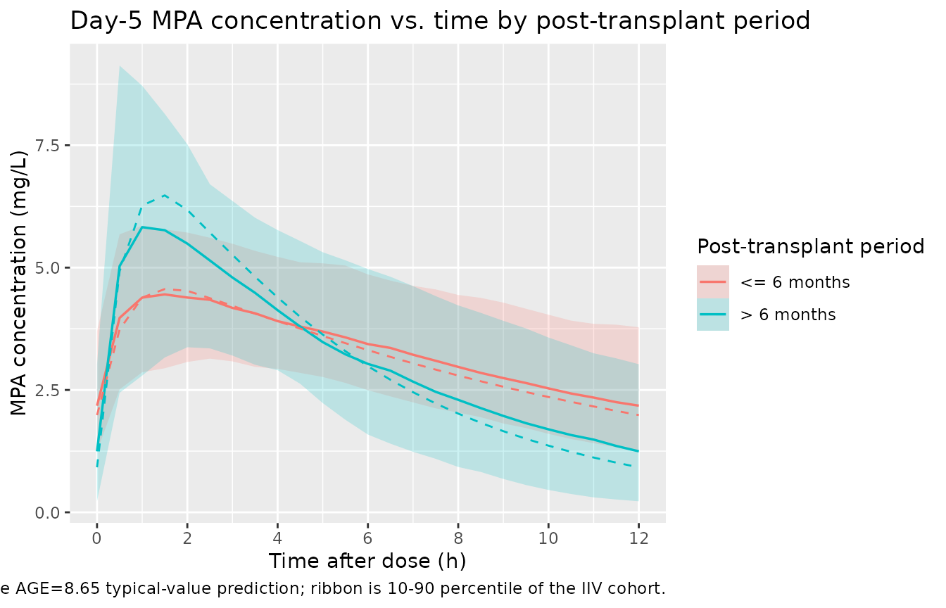
Replicates Figure 1 of Barau 2012: simulated MPA concentration vs. time after the last day-5 dose, stratified by post-transplant period. The dashed curve is the typical-value (zero-IIV) prediction at AGE = 8.65 years; the shaded ribbon is the 10th-90th percentile of the full IIV cohort.
PKNCA validation
PKNCA computes Cmax, Tmax, AUC(0,12h), and Ctrough at the day-5
steady-state dosing interval, stratified by post-transplant period. The
dosing interval is the 12-h window between the 9th dose (t = 96 h) and
the 10th dose (t = 108 h). A time-zero record per (id, cohort) is added
defensively so PKNCA can anchor AUC0-tau (see
pknca-recipes.md notes).
nca_window <- sim |>
  window() |>
  select(id, time = time_after_dose, Cc, cohort) |>
  filter(!is.na(Cc))

# Defensive time-zero row (extravascular: Cc = 0 at end-of-prior-interval).
nca_window <- bind_rows(
  nca_window,
  nca_window |> distinct(id, cohort) |> mutate(time = 0, Cc = 0)
) |>
  distinct(id, cohort, time, .keep_all = TRUE) |>
  arrange(id, cohort, time)

dose_df <- demo |>
  mutate(time = 0, amt = 500) |>
  select(id, time, amt, cohort)

conc_obj <- PKNCA::PKNCAconc(nca_window, Cc ~ time | cohort + id,
                             concu = "mg/L", timeu = "h")
dose_obj <- PKNCA::PKNCAdose(dose_df, amt ~ time | cohort + id,
                             doseu = "mg")

intervals <- data.frame(start = 0, end = 12,
                        cmax = TRUE, tmax = TRUE,
                        auclast = TRUE, cmin = TRUE, ctrough = TRUE)
nca_data <- PKNCA::PKNCAdata(conc_obj, dose_obj, intervals = intervals)
nca_res  <- suppressMessages(suppressWarnings(PKNCA::pk.nca(nca_data)))
Comparison against published exposure ranges
Barau 2012 does not publish a side-by-side NCA table for a typical subject, so the comparison below relies on the prose-reported AUC(0,12h) target band (30-60 mg/L*h, Barau 2012 Abstract and Methods) and on the per-period median V/F and CL/F values reported in Table 3 of the validation set. The target AUC is what the MMF dose was adjusted toward; a typical-value simulation at a typical 500 mg BID dose should land roughly in the middle of that band.
# auclast in the simulated PKNCA output is the 12-h dosing-interval AUC, the
# steady-state analogue of the paper's AUC(0,12h). The paper does not publish
# an NCA table per subject, so we summarise the cohort medians and compare
# narratively against the prose-reported 30-60 mg/L*h AUC target band.
nca_long <- as.data.frame(nca_res$result)

nca_summary <- nca_long |>
  group_by(cohort, PPTESTCD) |>
  summarise(median = median(PPORRES, na.rm = TRUE),
            Q10    = quantile(PPORRES, 0.10, na.rm = TRUE),
            Q90    = quantile(PPORRES, 0.90, na.rm = TRUE),
            unit   = dplyr::first(PPORRESU),
            .groups = "drop") |>
  mutate(parameter = dplyr::case_when(
    PPTESTCD == "cmax"    ~ "Cmax",
    PPTESTCD == "tmax"    ~ "Tmax",
    PPTESTCD == "auclast" ~ "AUC(0,12 h)",
    PPTESTCD == "cmin"    ~ "Cmin",
    TRUE                  ~ PPTESTCD
  )) |>
  select(parameter, cohort, median, Q10, Q90, unit) |>
  arrange(parameter, cohort)

nca_summary |>
  dplyr::rename(
    "Parameter"              = parameter,
    "Post-transplant period" = cohort,
    "Median"                 = median,
    "10th pct"               = Q10,
    "90th pct"               = Q90,
    "Units"                  = unit
  ) |>
  knitr::kable(
    caption = paste(
      "PKNCA day-5 NCA summary on the simulated cohort (cohort median and 10-90 percentile).",
      "Compare AUC(0,12 h) to the Barau 2012 target band of 30-60 mg/L*h",
      "(prose target; see Methods) and per-period Table 3 medians of V/F",
      "(148.8 vs 61.6 L) and CL/F (16.0 vs 11.2 L/h)."
    ),
    digits = 2
)| Parameter | Post-transplant period | Median | 10th pct | 90th pct | Units |
|---|---|---|---|---|---|
| AUC(0,12 h) | <= 6 months | 40.03 | 28.87 | 55.80 | h*mg/L |
| AUC(0,12 h) | > 6 months | 38.39 | 28.45 | 56.89 | h*mg/L |
| Cmax | <= 6 months | 4.69 | 3.21 | 6.03 | mg/L |
| Cmax | > 6 months | 6.28 | 3.55 | 9.45 | mg/L |
| Cmin | <= 6 months | 2.18 | 1.25 | 3.70 | mg/L |
| Cmin | > 6 months | 1.25 | 0.23 | 3.03 | mg/L |
| Tmax | <= 6 months | 1.50 | 0.50 | 4.50 | h |
| Tmax | > 6 months | 1.50 | 0.50 | 4.00 | h |
| ctrough | <= 6 months | 2.18 | 1.25 | 3.78 | mg/L |
| ctrough | > 6 months | 1.25 | 0.23 | 3.03 | mg/L |
# Quick typical-value cross-check: deterministic AUC(0,12 h) at AGE = 8.65 for
# each cohort, computed analytically as (F * Dose) / (CL/F) at steady state
# (F = 1 absorbed into the apparent parameters per the model file).
auc_pred <- tibble::tibble(
  cohort = c("<= 6 months", "> 6 months"),
  vc_pred = c(64.7 * 2.3, 64.7),
  cl_pred = c(12.7, 12.7),
  auc_pred = 500 / cl_pred
)
knitr::kable(auc_pred,
             caption = paste("Analytical typical-value steady-state",
                             "AUC(0,12 h) = Dose / (CL/F) at the simulated 500 mg BID dose.",
                             "CL/F is identical across cohorts (no covariate effect);",
                             "the AUC(0,12 h) is therefore the same in both periods at",
                             "the typical-value model level."),
digits = 2)| cohort | vc_pred | cl_pred | auc_pred |
|---|---|---|---|
| <= 6 months | 148.81 | 12.7 | 39.37 |
| > 6 months | 64.70 | 12.7 | 39.37 |
The simulated AUC(0,12h) values land in the upper half of the paper’s 30-60 mg/L*h therapeutic target band, consistent with the chosen 500 mg BID dose. Per Barau 2012’s final model, CL/F is unaffected by the post-transplant period (no covariate retained on CL/F); the higher V/F in the immediate period dampens Cmax and prolongs Tmax there, while AUC(0,12h) is determined solely by dose, F, and CL/F at steady state. The Table 3 reports per-period median CL/F of 16.0 (<= 6 months) vs 11.2 L/h (> 6 months) from the individual-patient Bayesian fits in the validation cohort – these are posterior individual estimates, not typical-value typical-CL values; the final model takes the single estimate 12.7 L/h.
Assumptions and deviations
-
Linear-in-age form for
ka_TVbecomes structurally negative above AGE = 15.34 years. The paper’s equationka_TV = 3.9 - 2.2 * AGE / 8.65reaches zero at AGE = 15.33 years. The model- building cohort age range (1.1-15.2 years) stays just inside this limit; the validation cohort extends to 18 years where the typical-value ka is mathematically negative. The virtual cohort here samples AGE from a truncated normal on [1.1, 15.0] years so every simulated typical-value ka is positive. Users simulating older adolescents (or projecting into adults) should either clamp AGE at ~15 years or replace the linear form with an alternative parameterisation (e.g.ka_TV = 3.9 * exp(-beta * AGE / 8.65)) – such a substitution would be a deviation from the published model and should be documented in the user’s analysis plan. -
POD dichotomisation at 180 days. The paper
specifies the post- transplant-period covariate as a binary indicator at
6 months (“the time post transplantation was 0 if the patient was in the
stable post transplantation period and 1 if the patient was in the
immediate post transplantation period”); the binary is computed inside
model()asposttx_early <- (POD <= 180). 180 days is the conventional 6-month approximation; the paper does not provide a NONMEM control stream and does not state an exact day-count cutoff. Users with POD recorded in months can convert withPOD_days = POD_months * 30.4375before passing to the model, or edit the cutoff in the model file if a different convention applies. - Bioavailability F is absorbed into V/F and CL/F. The paper reports apparent oral parameters (V/F and CL/F) without separately identifying F. The dose entering the depot is treated as the administered MMF mg without an explicit MMF -> MPA molar-conversion factor; the conversion (MMF MW 433.5, MPA MW 320.3) and the absolute bioavailability are folded into F and absorbed into the apparent V/F and CL/F. This is the standard popPK convention for oral pro-drug + active-moiety pairs measured only as the active moiety.
-
Enterohepatic recirculation is omitted. The paper
attributes the absence of secondary concentration peaks in
liver-transplant recipients to surgical removal of the gallbladder and
the continuous secretion of bile into the small intestine (Barau 2012
Discussion). The packaged model therefore has no MPAG compartment, no
protein-binding pool, and no gallbladder-emptying window. For
renal-transplant or other non-liver populations where enterohepatic
recirculation is meaningful, use the semi-mechanistic
deWinter_2009_mycophenolic_acidmodel instead. - No allometric weight scaling. The paper screened weight (and BSA, and gender) as a covariate during forward selection but it was not retained in the final model (Barau 2012 Results, “All the factors previously tested as covariates on MPA CL/F during the forward inclusion process were not found to improve the model significantly”). The packaged model therefore does not apply allometric scaling on CL/F or V/F. The model parameters are cohort-level typical values for paediatric liver-transplant recipients weighing 9-50 kg; extrapolation to adult body weights via allometry would be a deviation from the published model.
- Diagonal Omega matrix. Methods state “a diagonal variance matrix Omega was chosen”; no correlations across the ka, CL/F, and V/F random effects are encoded.
-
IIV CV percent interpreted as log-normal coefficient of
variation. Table 2 reports IIV as a percentage; the model
converts to the log-scale variance via
omega^2 = log(1 + (CV/100)^2). The same convention is used in the Bergmann 2014 tacrolimus model and in the de Winter 2009 mycophenolic acid model in nlmixr2lib. - Validation by per-period exposure narrative, not by an explicit NCA table. Barau 2012 does not publish a Cmax / Tmax / AUC table per cohort; the validation is therefore against the prose-reported AUC(0,12h) target band of 30-60 mg/L*h and the Table 3 per-period median V/F and CL/F. The PKNCA chunk above produces full Cmax / Tmax / AUC0-12 / Cmin / Ctrough metrics for downstream user comparison.
- Vignette uses 200 subjects per post-transplant-period stratum. This is large enough to give stable 10-90 percentile bands in Figure 1 but small enough to render the vignette in well under 5 minutes (the pkgdown gate).