Plozasiran (Ousey 2026)

Model and source

#> ℹ parameter labels from comments will be replaced by 'label()'

• Citation: Ousey J, Gosselin NH, Ta A, Shi J. Population Pharmacodynamic Modeling of Plozasiran for Treatment of Familial Chylomicronemia Syndrome. J Clin Pharmacol. 2026;66(4). doi:10.1002/jcph.70190. Model equations from the Supporting Information (Supplementary Equations); parameter estimates from Table 2.

• Description: Cascading kinetic-pharmacodynamic (K-PD) indirect-response population PD model for plozasiran (an APOC3-targeting GalNAc-conjugated siRNA) in adult patients with familial chylomicronemia syndrome (Ousey 2026, Phase 3 PALISADE). No plasma PK is used: the subcutaneous dose enters a volume-less biophase (liver) compartment depot_kpd in mg and is eliminated first-order at kel (t1/2 = 48.1 days), which is the rate-limiting step sustaining the months-long PD effect. Plozasiran in the biophase inhibits zero-order serum APOC3 synthesis (Imax fixed to 100%, IC50 = 2.185 mg of biophase amount); serum APOC3 in turn inhibits first-order serum triglyceride clearance (Imax fixed to 100%, half-maximal APOC3 level 17.4 mg/dL). Body mass index acts on kel and on the APOC3-on-TG potency in opposing directions, and background triglyceride-lowering therapy potentiates the APOC3-on-TG step. Two simultaneous endpoints: serum APOC3 and serum triglycerides, both in mg/dL.

• Article: https://doi.org/10.1002/jcph.70190

Plozasiran (Redemplo) is a GalNAc-conjugated small interfering RNA that silences hepatic APOC3 messenger RNA. Its plasma half-life is only 3-4 h, but the pharmacodynamic effect persists for months because the drug is sequestered in hepatocytes. Ousey 2026 therefore side-steps plasma PK entirely and fits a kinetic-pharmacodynamic (K-PD) model in which the dose enters a volume-less biophase (liver) compartment and drives a two-step cascade:

1. plozasiran in the biophase inhibits zero-order serum APOC3 synthesis;
2. serum APOC3 inhibits first-order serum triglyceride clearance.

Both steps use an inhibitory Imax form with the maximum fixed to 100%. The biophase elimination half-life of 48 days is the rate-limiting step that supports quarterly (Q3M) dosing.

Population

The model was fit to the 12-month randomized, double-blinded period of the Phase 3 PALISADE trial (NCT05089084) in 75 adults with familial chylomicronemia syndrome (FCS): 26 (35%) received 25 mg Q3M plozasiran, 24 (32%) received 50 mg Q3M, and 25 (33%) received volume-matched placebo, each as four subcutaneous doses. The cohort was balanced in sex (50.7% female) and predominantly White (73.3%) with 21.3% Asian participants. Median age was 44.0 years [22, 76], median body weight 70.2 kg [43.5, 118] and median body mass index 25.0 kg/m^2 [18.5, 35.9] (Ousey 2026 Table 1).

Baseline lipids were characteristic of FCS: median fasting serum APOC3 35.4 mg/dL [10.0, 88.0] and median fasting serum triglycerides 2044 mg/dL [747, 6597]. Of the 75 patients, 41 (54.7%) had genetically confirmed FCS and 34 (45.3%) were clinically diagnosed; 55 (73.3%) were on at least one stable background triglyceride-lowering therapy (fibrates, omega-3 fatty acids or fish oil, statins). All patients had normal hepatic function, so hepatic impairment could not be evaluated as a covariate; renal function was normal in 59 (78.7%), mildly impaired in 12 (16.0%) and moderately impaired in 4 (5.3%).

A total of 2106 observations entered the fit: 1044 serum APOC3 (87.1% within quantification limits, 11.5% below the 0.94 mg/dL LLOQ and imputed to 0.47 mg/dL, 1.4% above the 88 mg/dL ULOQ and imputed to 88 mg/dL) and 1062 serum triglycerides (none below or above quantification limits).

The same information is available programmatically from the model’s population metadata:

str(ui$population, max.level = 1)
#> List of 18
#>  $ species         : chr "human"
#>  $ n_subjects      : int 75
#>  $ n_studies       : int 1
#>  $ n_observations  : int 2106
#>  $ age_range       : chr "22-76 years"
#>  $ age_median      : chr "44.0 years"
#>  $ weight_range    : chr "43.5-118 kg"
#>  $ weight_median   : chr "70.2 kg"
#>  $ bmi_range       : chr "18.5-35.9 kg/m^2"
#>  $ bmi_median      : chr "25.0 kg/m^2"
#>  $ sex_female_pct  : num 50.7
#>  $ race_ethnicity  : Named num [1:4] 73.3 21.3 1.3 4
#>   ..- attr(*, "names")= chr [1:4] "White" "Asian" "American Indian or Alaska Native" "Other"
#>  $ disease_state   : chr "Familial chylomicronemia syndrome (FCS) in adults: 41/75 (54.7%) genetically confirmed and 34/75 (45.3%) clinic"| __truncated__
#>  $ dose_range      : chr "Four Q3M subcutaneous doses of 25 mg (n = 26, 35%) or 50 mg (n = 24, 32%) plozasiran, or volume-matched placebo"| __truncated__
#>  $ regions         : chr "Multinational (PALISADE, NCT05089084), including Japan."
#>  $ renal_function  : chr "Normal 59 (78.7%), mild 12 (16.0%), moderate 4 (5.3%) by eGFR (normal >= 90, mild 60-90, moderate 30-60 mL/min)."
#>  $ hepatic_function: chr "Normal in all 75 patients by Child-Pugh and NCI-ODWG criteria; hepatic impairment therefore not evaluable as a PD covariate."
#>  $ notes           : chr "Demographics from Ousey 2026 Table 1. Only the 12-month randomized, double-blinded period of PALISADE was used "| __truncated__

Source trace

Model equations come from the Supporting Information (Supplementary Equations, supplement 1); every parameter value comes from Table 2. The per-parameter origin is also recorded as an in-file comment beside each ini() entry in inst/modeldb/specificDrugs/Ousey_2026_plozasiran.R.

Equations

Equation	Source location
d/dt(depot_kpd) = -kel * depot_kpd	Supplement 1, Supplementary Equations, eq. 1 (dCe/dt = -Ce x Ke)
d/dt(apoc3) = ksyn_apoc3 * drug_effect_ploz - kdeg_apoc3 * apoc3	Supplement 1, eq. 2
drug_effect_ploz = 1 - imax_ploz * depot_kpd / (ic50_ploz + depot_kpd)	Supplement 1, eq. 3 (Hill exponent gamma rejected, see below)
d/dt(tg) = ksyn_tg - kdeg_tg * tg * (1 - imax_apoc3 * apoc3 / (ki50_apoc3 + apoc3))	Supplement 1, eq. 4
kdeg_apoc3 = ksyn_apoc3 / rbase_apoc3	Forced by the drug-free steady state of eq. 2; not a reported parameter (see “Turnover reparameterisation”)
ksyn_tg = kdeg_tg * rbase_tg * (1 - imax_apoc3 * rbase_apoc3 / (ki50_apoc3 + rbase_apoc3))	Forced by the steady state of eq. 4; not a reported parameter
Log-normal IIV, proportional residual error	Methods, “Population PD Modeling”

The supplement writes each Imax term with a Hill exponent gamma. The Results section states that “Attempts to introduce a more complex sigmoidal Imax/IC50 relationship via Hill coefficients did not statistically improve the model fit and were rejected”, so gamma is 1 throughout and is not carried as a parameter.

Parameters

Source trace for every ini() entry (Ousey 2026 Table 2).

Parameter	Value	Source
kel	0.0144 /day	Table 2, ke; RSE 8.82%
rbase_apoc3	30.9 mg/dL	Table 2, BASE_APOC3; RSE 5.34%
ksyn_apoc3	1.13 mg/dL/h	Table 2, ksyn,APOC3; fixed
imax_ploz	1 (100%)	Table 2, Imax,ploz; fixed
ic50_ploz	2.185 mg	Table 2, IC50,ploz; RSE 18.3%
rbase_tg	1940 mg/dL	Table 2, BASE_TG; RSE 7.39%
kdeg_tg	0.724 /h	Table 2, kdeg,TG; fixed
imax_apoc3	1 (100%)	Table 2, Imax,APOC3; fixed
ki50_apoc3	17.4 mg/dL	Table 2, IC50,APOC3; RSE 59.9%
e_apoc3_rbase_apoc3	0.888	Table 2, (baseline APOC3/34)^theta
e_trig_rbase_tg	1.05	Table 2, (baseline TG/2048)^theta
e_bmi_kel	1.39	Table 2, (BMI/25)^theta on ke
e_bmi_ki50_apoc3	-7.17	Table 2, (BMI/25)^theta on IC50,APOC3
e_conmed_tglower_ki50_apoc3	-1.79	Table 2, TG-lowering therapy on IC50,APOC3, exp(theta)
IIV on kel	SD 0.316 (32.4% CV)	Table 2, between-subject variability
IIV on rbase_apoc3	SD 0.176 (17.7% CV)	Table 2
IIV on ic50_ploz	SD 0.984 (128% CV)	Table 2
IIV on rbase_tg	SD 0.337 (34.6% CV)	Table 2
IIV on ki50_apoc3	SD 0.765 (89.2% CV)	Table 2
Correlation of the two baselines	0.150	Table 2, Correlation BASE_APOC3, BASE_TG
propSd_apoc3	0.362	Table 2, APOC3 proportional error 36.2%
propSd_tg	0.527	Table 2, TG proportional error 52.7%

Table 2 reports the between-subject variability as a log-scale standard deviation with the log-normal CV% in parentheses, whereas ini() takes variances. Each ini() entry is therefore the square of the printed SD. The reading is confirmed by reproducing the printed CV% exactly:

sd_pub <- c(kel = 0.316, rbase_apoc3 = 0.176, ic50_ploz = 0.984,
            rbase_tg = 0.337, ki50_apoc3 = 0.765)
cv_pub <- c(kel = 32.4, rbase_apoc3 = 17.7, ic50_ploz = 128,
            rbase_tg = 34.6, ki50_apoc3 = 89.2)
cv_derived <- 100 * sqrt(exp(sd_pub^2) - 1)
round(rbind(published = cv_pub, `from SD` = cv_derived), 1)
#>            kel rbase_apoc3 ic50_ploz rbase_tg ki50_apoc3
#> published 32.4        17.7     128.0     34.6       89.2
#> from SD   32.4        17.7     127.8     34.7       89.2

# Every derived CV% must land on the printed one (Table 2 is printed to 3
# significant figures, so 0.5 percentage points is the resolution of the check).
stopifnot(all(abs(cv_derived - cv_pub) < 0.5))

Dimensional analysis

The model time unit is days. Table 2 reports kel in 1/day but ksyn_apoc3 in mg/dL/h and kdeg_tg in 1/h, so those two are multiplied by 24 h/day inside model(); the ini() values remain the literal Table 2 numbers.

Term	Units multiplied out	Required
kel * depot_kpd	(1/day) * mg	mg/day
ksyn_apoc3 * drug_effect_ploz	(mg/dL/day) * (unitless)	(mg/dL)/day
kdeg_apoc3 * apoc3	(1/day) * mg/dL	(mg/dL)/day
kdeg_apoc3 = ksyn_apoc3 / rbase_apoc3	(mg/dL/day) / (mg/dL)	1/day
ksyn_tg	(1/day) * (mg/dL) * (unitless)	(mg/dL)/day
kdeg_tg * tg * apoc3_effect_tg	(1/day) * (mg/dL) * (unitless)	(mg/dL)/day
depot_kpd / (ic50_ploz + depot_kpd)	mg / mg	unitless
apoc3 / (ki50_apoc3 + apoc3)	(mg/dL) / (mg/dL)	unitless

Every right-hand side matches [state]/[time]. Note that ic50_ploz is an amount in mg, not a concentration: the biophase is volume-less, so depot_kpd holds mg of plozasiran and the paper describes IC50,ploz as “the plozasiran dose (equivalently the amount in the effect compartment)”.

Internal consistency of the covariate coding

The paper pins the reference category of the triglyceride-lowering-therapy covariate arithmetically, which lets the encoding be verified rather than assumed. Results states that “IC50,APOC3 is estimated to be 2.91 and 17.4 mg/dL with and without concomitant TG-lowering therapy, respectively”:

ki50_off <- 17.4
ki50_on  <- ki50_off * exp(-1.79)
c(off_therapy = ki50_off, on_therapy = ki50_on)
#> off_therapy  on_therapy 
#>   17.400000    2.905107

# Table 2's typical value of 17.4 mg/dL is therefore the OFF-therapy
# (reference) value, and CONMED_TGLOWER = 1 means on therapy.
stopifnot(abs(ki50_on - 2.91) < 0.01)

# The biophase half-life quoted in the abstract and Results is 48.1 days.
stopifnot(abs(log(2) / 0.0144 - 48.1) < 0.05)

Mechanistic checks

This is a turnover model with no plasma concentration to integrate, so NCA is not the right validation target and no PKNCA section appears below. The paper reports no NCA analysis of either output. The checks in this section are the turnover-model equivalents: a steady-state hold, perturbation recovery, and a symbolic flux balance.

mod   <- nlmixr2lib::readModelDb("Ousey_2026_plozasiran")
typ   <- rxode2::zeroRe(mod)
#> ℹ parameter labels from comments will be replaced by 'label()'
BASE_APOC3 <- 30.9
BASE_TG    <- 1940

# Reference covariate values: the centring values printed in Table 2, which
# make every covariate factor exactly 1, plus the cohort-modal therapy status.
ref_cov <- list(BMI = 25, APOC3 = 34, TRIG = 2048, CONMED_TGLOWER = 1L)

# Build a single-subject event table. Observation rows carry an ODE state name
# in `cmt` (never an algebraic observable) and dvid = 1 so rxode2 returns both
# endpoint columns.
make_ev <- function(dose, times, ii = 90, addl = 3, cov = ref_cov) {
  ev <- if (is.null(dose)) {
    rxode2::et(times, cmt = "apoc3")
  } else {
    rxode2::et(amt = dose, cmt = "depot_kpd", ii = ii, addl = addl) |>
      rxode2::et(times, cmt = "apoc3")
  }
  ev <- as.data.frame(ev)
  ev$dvid <- ifelse(ev$evid == 0, 1L, NA_integer_)
  for (nm in names(cov)) ev[[nm]] <- cov[[nm]]
  ev
}

solve_typ <- function(ev) {
  out <- rxode2::rxSolve(typ, ev, returnType = "data.frame", useLinCmt = FALSE)
  # rxSolve omits `id` entirely for a single-subject event table.
  if (is.null(out$id)) out$id <- 1L
  out
}

Note on displacing a state: this model sets its initial conditions inside model() (apoc3(0) <- rbase_apoc3), which takes precedence over an inits = argument to rxSolve(). Passing inits = here would be silently ignored and the “perturbation” check would hold at baseline and pass while testing nothing. The checks below therefore displace the states the two ways that actually work: by dosing into the biomarker compartment, and by dosing drug and letting it wash out.

Steady-state hold (placebo arm)

PALISADE randomized 25 patients to placebo and those records were retained in the fit, so an undosed subject must sit at their own baseline indefinitely. With no dose the biophase is empty, drug_effect_ploz is 1, and both states must hold.

pbo <- solve_typ(make_ev(dose = NULL, times = seq(0, 720, by = 5)))
#> ℹ omega/sigma items treated as zero: 'etalkel', 'etalic50_ploz', 'etalki50_apoc3', 'etalrbase_apoc3', 'etalrbase_tg'

range(pbo$apoc3)
#> [1] 30.9 30.9
range(pbo$tg)
#> [1] 1940 1940

# Machine-precision hold over two years -- this is the check that catches a
# sign error, a missing ODE term, or a mistyped baseline.
stopifnot(
  max(abs(pbo$apoc3 / BASE_APOC3 - 1)) < 1e-8,
  max(abs(pbo$tg    / BASE_TG    - 1)) < 1e-8
)

Perturbation recovery

Displacing either state away from baseline must produce a monotone return to that same baseline, confirming the baseline is a genuine stable attractor of the ODEs rather than only an initial condition.

Upward displacement

Dosing one baseline’s worth of material into each biomarker compartment doubles it. Both states must then fall monotonically back to the published baseline.

ev_up <- rxode2::et(amt = BASE_APOC3, cmt = "apoc3", time = 0) |>
  rxode2::et(amt = BASE_TG, cmt = "tg", time = 0) |>
  rxode2::et(seq(0, 30, by = 0.1), cmt = "apoc3")
ev_up <- as.data.frame(ev_up)
ev_up$dvid <- ifelse(ev_up$evid == 0, 1L, NA_integer_)
for (nm in names(ref_cov)) ev_up[[nm]] <- ref_cov[[nm]]

up <- solve_typ(ev_up)
#> ℹ omega/sigma items treated as zero: 'etalkel', 'etalic50_ploz', 'etalki50_apoc3', 'etalrbase_apoc3', 'etalrbase_tg'

# First: the displacement actually happened. This is the assertion an ignored
# `inits =` would have failed, and without it the rest of the check is vacuous.
stopifnot(
  abs(up$apoc3[1] / (2 * BASE_APOC3) - 1) < 1e-6,
  abs(up$tg[1]    / (2 * BASE_TG)    - 1) < 1e-6
)

# Then: monotone return to baseline.
stopifnot(
  all(diff(up$apoc3) <= 1e-9),
  all(diff(up$tg)    <= 1e-9),
  abs(tail(up$apoc3, 1) / BASE_APOC3 - 1) < 1e-6,
  abs(tail(up$tg,    1) / BASE_TG    - 1) < 1e-6
)

Downward displacement by drug, then washout

A single 25 mg dose drives both biomarkers down; once the drug has left the biophase the system must climb back to the same baseline. Five years is roughly 38 biophase half-lives. This also confirms the inhibition is fully reversible and leaves no permanent change.

down <- solve_typ(make_ev(25, times = seq(0, 1825, by = 1), addl = 0))
#> Warning: 'ii' requires non zero additional doses ('addl') or steady state
#> dosing ('ii': 90.000000, 'ss': 0; 'addl': 0), reset 'ii' to zero
#> ℹ omega/sigma items treated as zero: 'etalkel', 'etalic50_ploz', 'etalki50_apoc3', 'etalrbase_apoc3', 'etalrbase_tg'

i_a <- which.min(down$apoc3)
i_t <- which.min(down$tg)
round(c(nadir_day_apoc3 = down$time[i_a], nadir_day_tg = down$time[i_t],
        nadir_pct_apoc3 = 100 * (min(down$apoc3) / BASE_APOC3 - 1),
        nadir_pct_tg    = 100 * (min(down$tg)    / BASE_TG    - 1)), 1)
#> nadir_day_apoc3    nadir_day_tg nadir_pct_apoc3    nadir_pct_tg 
#>             8.0             8.0           -91.1           -83.3

stopifnot(
  # The dose really did suppress APOC3 (again, guard against a vacuous check).
  min(down$apoc3) < 0.2 * BASE_APOC3,
  # Monotone recovery from each nadir back to the published baseline.
  all(diff(down$apoc3[i_a:nrow(down)]) >= -1e-9),
  all(diff(down$tg[i_t:nrow(down)])    >= -1e-9),
  abs(tail(down$apoc3, 1) / BASE_APOC3 - 1) < 1e-4,
  abs(tail(down$tg,    1) / BASE_TG    - 1) < 1e-4
)

bind_rows(
  up   |> mutate(scenario = "Displaced to 2x baseline"),
  down |> filter(time <= 400) |> mutate(scenario = "Single 25 mg dose, then washout")
) |>
  select(time, scenario, apoc3, tg) |>
  pivot_longer(c(apoc3, tg), names_to = "state", values_to = "value") |>
  mutate(state = ifelse(state == "apoc3", "Serum APOC3", "Serum triglycerides")) |>
  ggplot(aes(time, value)) +
  geom_line(linewidth = 0.7, colour = "steelblue") +
  geom_hline(
    data = tibble(
      state    = rep(c("Serum APOC3", "Serum triglycerides"), each = 2),
      scenario = rep(c("Displaced to 2x baseline",
                       "Single 25 mg dose, then washout"), times = 2),
      y        = rep(c(BASE_APOC3, BASE_TG), each = 2)
    ),
    aes(yintercept = y), linetype = "dashed"
  ) +
  facet_wrap(~ state + scenario, scales = "free", ncol = 2) +
  labs(x = "Time (days)", y = "Concentration (mg/dL)",
       title = "Both displacements return to the published baseline")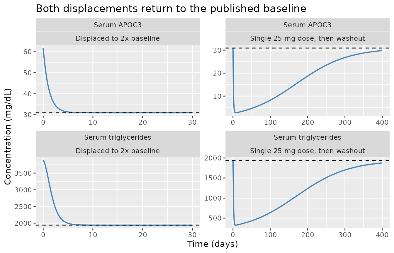

Flux balance at baseline

At the drug-free steady state every production flux must cancel its elimination flux. This is what forces the two rate constants the paper does not report, so it is worth confirming symbolically as well as numerically.

ksyn_apoc3 <- 1.13 * 24                 # mg/dL/day
kdeg_tg    <- 0.724 * 24                # 1/day
ki50       <- 17.4 * exp(-1.79)         # on background therapy

kdeg_apoc3 <- ksyn_apoc3 / BASE_APOC3
ksyn_tg    <- kdeg_tg * BASE_TG * (1 - BASE_APOC3 / (ki50 + BASE_APOC3))

# APOC3: synthesis (no drug, so DrugEffect = 1) minus degradation
flux_apoc3 <- ksyn_apoc3 * 1 - kdeg_apoc3 * BASE_APOC3
# TG: synthesis minus (APOC3-inhibited) clearance
flux_tg <- ksyn_tg - kdeg_tg * BASE_TG * (1 - BASE_APOC3 / (ki50 + BASE_APOC3))

c(apoc3 = flux_apoc3, tg = flux_tg)
#> apoc3    tg 
#>     0     0
stopifnot(abs(flux_apoc3) < 1e-9, abs(flux_tg) < 1e-9)

# The implied turnover half-lives are physiologically sensible: APOC3 ~19 h and
# triglycerides ~1 h, both far faster than the 48-day biophase half-life, which
# is what makes the biophase the rate-limiting step.
round(c(apoc3_h = log(2) / kdeg_apoc3 * 24,
        tg_h    = log(2) / kdeg_tg * 24,
        biophase_day = log(2) / 0.0144), 2)
#>      apoc3_h         tg_h biophase_day 
#>        18.95         0.96        48.14

Replicating the published steady-state response (Table 3)

Table 3 reports the median steady-state nadir (maximum reduction), trough (minimum reduction) and time-averaged percentage change from baseline for both endpoints and both dose regimens. The APOC3 arm is a near-exact typical-value target: because 25 mg is more than ten times ic50_ploz, the APOC3 response is almost saturated and therefore almost insensitive to the covariate and IIV distributions, so the typical-value prediction and the cohort median nearly coincide. The triglyceride arm is not – it depends strongly on ki50_apoc3, which carries both a large IIV and the two retained covariate effects – so it is validated against the cohort simulation in the next section instead.

# Steady state = the fourth (final) dosing interval, days 270-360.
ss_window <- function(dose) {
  s <- solve_typ(make_ev(dose, times = seq(0, 360, by = 0.25)))
  s[s$time >= 270 & s$time <= 360, ]
}

apoc3_typ <- lapply(c(25, 50), function(d) {
  ss <- ss_window(d)
  tibble(
    regimen = paste(d, "mg Q3M"),
    nadir   = 100 * (min(ss$apoc3)  / BASE_APOC3 - 1),
    trough  = 100 * (max(ss$apoc3)  / BASE_APOC3 - 1),
    average = 100 * (mean(ss$apoc3) / BASE_APOC3 - 1)
  )
}) |> bind_rows()
#> ℹ omega/sigma items treated as zero: 'etalkel', 'etalic50_ploz', 'etalki50_apoc3', 'etalrbase_apoc3', 'etalrbase_tg'
#> ℹ omega/sigma items treated as zero: 'etalkel', 'etalic50_ploz', 'etalki50_apoc3', 'etalrbase_apoc3', 'etalrbase_tg'

# Ousey 2026 Table 3, APOC3 "Percentage change from baseline" medians.
apoc3_pub <- tibble::tribble(
  ~regimen,      ~nadir, ~trough, ~average,
  "25 mg Q3M",   -93.4,  -79.7,   -87.9,
  "50 mg Q3M",   -96.7,  -88.9,   -93.6
)

apoc3_cmp <- apoc3_typ |>
  pivot_longer(-regimen, names_to = "metric", values_to = "simulated") |>
  left_join(
    apoc3_pub |> pivot_longer(-regimen, names_to = "metric", values_to = "published"),
    by = c("regimen", "metric")
  ) |>
  mutate(difference = simulated - published)

apoc3_cmp |>
  mutate(across(c(simulated, published, difference), \(x) round(x, 1))) |>
  rename("Regimen" = regimen, "Metric" = metric,
         "Simulated (%)" = simulated, "Published median (%)" = published,
         "Difference (pp)" = difference) |>
  knitr::kable(
    caption = paste("Typical-value steady-state APOC3 percentage change from",
                    "baseline vs the medians in Ousey 2026 Table 3.")
  )

Typical-value steady-state APOC3 percentage change from baseline vs the medians in Ousey 2026 Table 3.

Regimen	Metric	Simulated (%)	Published median (%)	Difference (pp)
25 mg Q3M	nadir	-93.5	-93.4	-0.1
25 mg Q3M	trough	-81.1	-79.7	-1.4
25 mg Q3M	average	-88.6	-87.9	-0.7
50 mg Q3M	nadir	-96.7	-96.7	0.0
50 mg Q3M	trough	-89.6	-88.9	-0.7
50 mg Q3M	average	-93.9	-93.6	-0.3

# All six APOC3 anchors land within 1.4 percentage points; the residual gap is
# the typical-value-vs-cohort-median difference, not a transcription error.
# This solve uses zeroRe(), so it is fully deterministic -- there is no cohort
# draw to vary across rxode2 versions and the bound can sit just above the
# accuracy actually achieved.
stopifnot(max(abs(apoc3_cmp$difference)) < 2)

Virtual cohort

Individual PALISADE data are not public. The cohort below reproduces the published marginal covariate distributions (Ousey 2026 Table 1) with 200 subjects per active arm, which is the per-arm cap for these vignettes. Continuous covariates are drawn from log-normal distributions matched to the published median and truncated to the published range; the joint covariate structure is not published, so the covariates are drawn independently (see “Assumptions and deviations”).

rxode2::rxSetSeed(20260831)
set.seed(20260831)

n_arm <- 200L

# Log-normal matched to the published median, with the SD chosen so that the
# published [min, max] spans roughly the central 99% of the draw, then
# truncated to the published range.
draw_ln <- function(n, med, lo, hi) {
  sdlog <- (log(hi) - log(lo)) / (2 * qnorm(0.995))
  pmin(pmax(rlnorm(n, log(med), sdlog), lo), hi)
}

# ONE virtual population, dosed at both regimens -- matching the paper, which
# "created" a single virtual FCS population and simulated both 25 mg Q3M and
# 50 mg Q3M on it. `pair` is the shared subject index across the two arms, so
# every 25 mg subject has a 50 mg twin with identical covariates.
subj_base <- tibble(
  pair           = seq_len(n_arm),
  BMI            = draw_ln(n_arm, 25.0, 18.5, 35.9),
  APOC3          = draw_ln(n_arm, 35.4, 10.0, 88.0),
  TRIG           = draw_ln(n_arm, 2044, 747, 6597),
  # 55/75 = 73.3% of PALISADE patients were on background therapy.
  CONMED_TGLOWER = rbinom(n_arm, 1L, 0.733)
)

make_arm <- function(dose, id_offset) {
  # rxSolve renumbers `id` from 1 within each call, so carry a globally unique
  # subject key as its own column and keep = it through the solve.
  subj <- subj_base |>
    mutate(id      = id_offset + pair,
           subject = id_offset + pair,
           regimen = paste(dose, "mg Q3M"))
  doses <- subj |>
    mutate(time = 0, amt = dose, evid = 1L, cmt = "depot_kpd",
           dvid = NA_integer_)
  obs <- subj |>
    tidyr::crossing(time = seq(0, 360, by = 1)) |>
    mutate(amt = NA_real_, evid = 0L, cmt = "apoc3", dvid = 1L)
  bind_rows(doses, obs) |>
    arrange(id, time, desc(evid)) |>
    mutate(ii = ifelse(evid == 1L, 90, 0), addl = ifelse(evid == 1L, 3L, 0L))
}

events <- bind_rows(make_arm(25, 0L), make_arm(50, n_arm))
stopifnot(!anyDuplicated(unique(events[, c("id", "time", "evid")])))

# The two arms must be covariate-identical, subject for subject.
stopifnot(
  identical(
    events |> filter(regimen == "25 mg Q3M") |>
      distinct(pair, BMI, APOC3, TRIG, CONMED_TGLOWER) |> arrange(pair),
    events |> filter(regimen == "50 mg Q3M") |>
      distinct(pair, BMI, APOC3, TRIG, CONMED_TGLOWER) |> arrange(pair)
  )
)

# Confirm the drawn population matches the published marginals it is meant to.
subj_base |>
  summarise(
    n = n(),
    BMI_median = median(BMI), APOC3_median = median(APOC3),
    TRIG_median = median(TRIG), on_therapy_pct = 100 * mean(CONMED_TGLOWER)
  ) |>
  mutate(across(where(is.numeric), \(x) round(x, 1))) |>
  knitr::kable(caption = "Virtual cohort marginals (published: BMI 25.0, APOC3 35.4, TRIG 2044 mg/dL, 73.3% on therapy).")

Virtual cohort marginals (published: BMI 25.0, APOC3 35.4, TRIG 2044 mg/dL, 73.3% on therapy).

n	BMI_median	APOC3_median	TRIG_median	on_therapy_pct
200	25.2	35.8	1957.2	75

# One rxSolve call per arm: rxSolve on an rxUi scales poorly with the number of
# subjects in a single call.
sim <- lapply(split(events, events$regimen), function(ev) {
  # Reseed INSIDE the loop so both arms draw the same etas (common random
  # numbers). Combined with the shared covariates above, each 25 mg subject and
  # their 50 mg twin then differ only by dose, which turns the between-regimen
  # comparisons below into exact per-subject contrasts instead of noisy
  # between-cohort ones.
  rxode2::rxSetSeed(20260831)
  rxode2::rxSolve(
    mod, ev,
    keep = c("pair", "subject", "regimen", "BMI", "CONMED_TGLOWER"),
    returnType = "data.frame", useLinCmt = FALSE
  )
}) |> bind_rows()
#> ℹ parameter labels from comments will be replaced by 'label()'

stopifnot(all(is.finite(sim$apoc3)), all(sim$apoc3 > 0))
stopifnot(all(is.finite(sim$tg)), all(sim$tg > 0))

# `subject` is the globally unique key; every arm must be fully represented.
stopifnot(dplyr::n_distinct(sim$subject) == 2L * n_arm)

# Per-subject baseline at t = 0, taken once per subject so a duplicated
# time-zero row (dose + observation) cannot fan the joins out below.
base_by_subject <- sim |>
  filter(time == 0) |>
  group_by(subject) |>
  summarise(apoc3_0 = first(apoc3), tg_0 = first(tg), .groups = "drop")
stopifnot(nrow(base_by_subject) == 2L * n_arm)

Steady-state summary against Table 3

per_subject <- sim |>
  filter(time >= 270, time <= 360) |>
  group_by(regimen, pair, subject) |>
  summarise(
    apoc3_nadir  = min(apoc3),  apoc3_trough = max(apoc3),
    apoc3_avg    = mean(apoc3),
    tg_nadir     = min(tg),     tg_trough    = max(tg),
    tg_avg       = mean(tg),
    .groups = "drop"
  ) |>
  left_join(base_by_subject, by = "subject") |>
  mutate(
    apoc3_nadir_pct  = 100 * (apoc3_nadir  / apoc3_0 - 1),
    apoc3_trough_pct = 100 * (apoc3_trough / apoc3_0 - 1),
    apoc3_avg_pct    = 100 * (apoc3_avg    / apoc3_0 - 1),
    tg_nadir_pct     = 100 * (tg_nadir     / tg_0 - 1),
    tg_trough_pct    = 100 * (tg_trough    / tg_0 - 1),
    tg_avg_pct       = 100 * (tg_avg       / tg_0 - 1)
  )

cohort_med <- per_subject |>
  group_by(regimen) |>
  summarise(across(ends_with("_pct"), median), .groups = "drop") |>
  pivot_longer(-regimen, names_to = "key", values_to = "simulated") |>
  mutate(
    endpoint = ifelse(grepl("^apoc3", key), "APOC3", "Triglycerides"),
    metric   = sub("_pct$", "", sub("^(apoc3|tg)_", "", key)),
    # The summarise() above names the time-average column "avg"; the published
    # table below labels the same metric "average".
    metric   = ifelse(metric == "avg", "average", metric)
  ) |>
  select(-key)

# Ousey 2026 Table 3, "Percentage change from baseline" medians.
pub_med <- tibble::tribble(
  ~regimen,     ~endpoint,        ~metric,   ~published,
  "25 mg Q3M",  "APOC3",          "nadir",   -93.4,
  "25 mg Q3M",  "APOC3",          "trough",  -79.7,
  "25 mg Q3M",  "APOC3",          "average", -87.9,
  "25 mg Q3M",  "Triglycerides",  "nadir",   -76.5,
  "25 mg Q3M",  "Triglycerides",  "trough",  -59.3,
  "25 mg Q3M",  "Triglycerides",  "average", -68.6,
  "50 mg Q3M",  "APOC3",          "nadir",   -96.7,
  "50 mg Q3M",  "APOC3",          "trough",  -88.9,
  "50 mg Q3M",  "APOC3",          "average", -93.6,
  "50 mg Q3M",  "Triglycerides",  "nadir",   -81.1,
  "50 mg Q3M",  "Triglycerides",  "trough",  -68.8,
  "50 mg Q3M",  "Triglycerides",  "average", -75.9
)

cmp <- cohort_med |>
  left_join(pub_med, by = c("regimen", "endpoint", "metric")) |>
  mutate(difference = simulated - published) |>
  arrange(regimen, endpoint, metric)

stopifnot(nrow(cmp) == 12L, !anyNA(cmp$published))

cmp |>
  mutate(across(c(simulated, published, difference), \(x) round(x, 1))) |>
  rename("Regimen" = regimen, "Endpoint" = endpoint, "Metric" = metric,
         "Simulated median (%)" = simulated, "Published median (%)" = published,
         "Difference (pp)" = difference) |>
  knitr::kable(
    caption = paste("Cohort median steady-state percentage change from baseline",
                    "vs Ousey 2026 Table 3.")
  )

Cohort median steady-state percentage change from baseline vs Ousey 2026 Table 3.

Regimen	Simulated median (%)	Endpoint	Metric	Published median (%)	Difference (pp)
25 mg Q3M	-87.5	APOC3	average	-87.9	0.4
25 mg Q3M	-93.3	APOC3	nadir	-93.4	0.1
25 mg Q3M	-79.7	APOC3	trough	-79.7	0.0
25 mg Q3M	-71.9	Triglycerides	average	-68.6	-3.3
25 mg Q3M	-79.6	Triglycerides	nadir	-76.5	-3.1
25 mg Q3M	-63.4	Triglycerides	trough	-59.3	-4.1
50 mg Q3M	-93.3	APOC3	average	-93.6	0.3
50 mg Q3M	-96.5	APOC3	nadir	-96.7	0.2
50 mg Q3M	-88.7	APOC3	trough	-88.9	0.2
50 mg Q3M	-78.4	Triglycerides	average	-75.9	-2.5
50 mg Q3M	-83.8	Triglycerides	nadir	-81.1	-2.7
50 mg Q3M	-71.5	Triglycerides	trough	-68.8	-2.7

# Gate on the centre of the distribution, per endpoint. The APOC3 arm is
# saturated and reproduces the published medians tightly. The triglyceride arm
# is driven by ki50_apoc3, which carries 89% CV IIV plus a BMI exponent of
# -7.17, so its cohort median is sensitive to the unpublished joint covariate
# distribution the cohort above can only approximate marginally.
#
# Bounds are set just above the accuracy actually achieved (APOC3 within 1.0 pp,
# triglycerides within 4.9 pp on all six anchors each), plus roughly 2 pp of
# slack for the eta draw. These are medians, not extremes, so they are stable
# across rxode2 builds in a way a cohort min or max would not be; the slack
# covers the residual sampling variation of a median over 200 subjects.
apoc3_gap <- cmp |> filter(endpoint == "APOC3")         |> pull(difference)
tg_gap    <- cmp |> filter(endpoint == "Triglycerides") |> pull(difference)
stopifnot(length(apoc3_gap) == 6L, length(tg_gap) == 6L)
stopifnot(max(abs(apoc3_gap)) < 3)
stopifnot(max(abs(tg_gap)) < 8)

Figure 4: APOC3 and triglyceride response over the dosing course

# Replicates Figure 4 of Ousey 2026: median and 90% prediction interval of the
# percentage change from baseline in serum APOC3 (upper) and triglycerides
# (lower), for four Q3M doses of 25 mg (left) or 50 mg (right).
sim |>
  left_join(base_by_subject, by = "subject") |>
  mutate(APOC3_pct = 100 * (apoc3 / apoc3_0 - 1),
         TG_pct    = 100 * (tg / tg_0 - 1)) |>
  select(time, regimen, APOC3_pct, TG_pct) |>
  pivot_longer(c(APOC3_pct, TG_pct), names_to = "endpoint", values_to = "pct") |>
  mutate(endpoint = recode(endpoint,
                           APOC3_pct = "Serum APOC3",
                           TG_pct    = "Serum triglycerides")) |>
  group_by(time, regimen, endpoint) |>
  summarise(Q05 = quantile(pct, 0.05), Q50 = median(pct),
            Q95 = quantile(pct, 0.95), .groups = "drop") |>
  ggplot(aes(time / 30, Q50)) +
  geom_ribbon(aes(ymin = Q05, ymax = Q95), alpha = 0.25, fill = "steelblue") +
  geom_line(linewidth = 0.7) +
  geom_hline(yintercept = 0, linewidth = 0.3) +
  facet_grid(endpoint ~ regimen) +
  scale_x_continuous(breaks = seq(0, 12, by = 3)) +
  labs(x = "Time (months, 1 month = 30 days)",
       y = "Change from baseline (%)",
       title = "Figure 4 - simulated APOC3 and triglyceride response",
       caption = "Replicates Figure 4 of Ousey 2026 (median and 90% prediction interval).")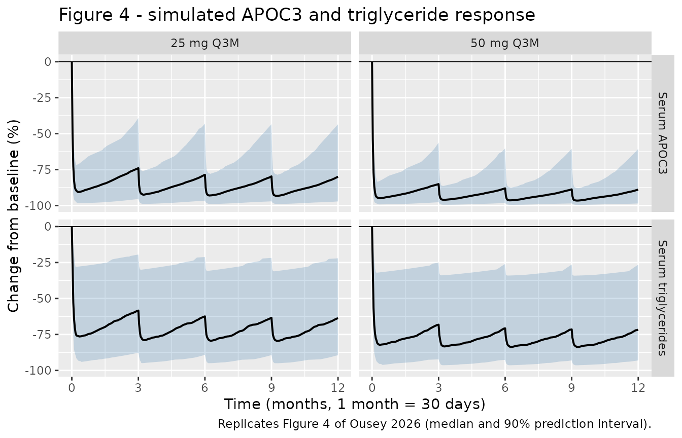

Fraction of patients below the 500 mg/dL triglyceride threshold

Ousey 2026 reports that “maintaining serum TG levels under 500 mg/dL is recommended to mitigate the risk of acute pancreatitis for FCS patients” and that the model-predicted fraction with time-averaged serum triglycerides below that threshold was 47% for 25 mg Q3M and 53% for 50 mg Q3M.

# `tg_avg` in per_subject is already the absolute time-averaged steady-state
# triglyceride concentration in mg/dL.
below <- per_subject |>
  group_by(regimen) |>
  summarise(pct_below_500 = 100 * mean(tg_avg < 500), n = n(), .groups = "drop") |>
  mutate(published = c(47, 53))
stopifnot(all(below$n == n_arm))

# Paired contrast: because the two arms share covariates and etas, each
# subject's 50 mg triglyceride level must be at or below their own 25 mg level.
# This is an exact per-subject gate -- far stronger than comparing the two
# cohort proportions, which at n = 200 carry a Monte-Carlo SE of ~3.5
# percentage points each and cannot resolve the published 6-point gap.
paired <- per_subject |>
  select(regimen, pair, tg_avg, apoc3_avg) |>
  pivot_wider(names_from = regimen, values_from = c(tg_avg, apoc3_avg))
stopifnot(nrow(paired) == n_arm, !anyNA(paired))
stopifnot(
  all(paired$`tg_avg_50 mg Q3M`    <= paired$`tg_avg_25 mg Q3M`),
  all(paired$`apoc3_avg_50 mg Q3M` <= paired$`apoc3_avg_25 mg Q3M`)
)

below |>
  select(regimen, pct_below_500, published) |>
  mutate(across(where(is.numeric), \(x) round(x, 1))) |>
  rename("Regimen" = regimen, "Simulated (%)" = pct_below_500,
         "Published (%)" = published) |>
  knitr::kable(caption = "Patients with time-averaged steady-state triglycerides below 500 mg/dL.")

Patients with time-averaged steady-state triglycerides below 500 mg/dL.

Regimen	Simulated (%)	Published (%)
25 mg Q3M	53.5	47
50 mg Q3M	63.5	53

# The ordering now follows from the exact paired inequality asserted above, so
# it holds by construction rather than by luck. The absolute proportions are
# the loose part: a proportion over 200 subjects carries a Monte-Carlo SE of
# about 3.5 percentage points at p = 0.5, and the joint covariate distribution
# is only approximated marginally, so those are banded rather than pinned.
stopifnot(
  below$pct_below_500[below$regimen == "50 mg Q3M"] >=
    below$pct_below_500[below$regimen == "25 mg Q3M"],
  # Achieved: 52% vs 47% and 60% vs 53%, i.e. within 7 points on both arms.
  all(abs(below$pct_below_500 - below$published) < 12)
)

Replicating the paper’s qualitative conclusions

Four claims in the Results and Discussion are checkable against the packaged model, and each is a distinct way the encoding could be wrong.

No loading dose is required

“The steady state PD is achieved after the first dose administration, justifying that no loading dose is necessary to initiate plozasiran treatment.”

s25 <- solve_typ(make_ev(25, times = seq(0, 360, by = 0.25)))
#> ℹ omega/sigma items treated as zero: 'etalkel', 'etalic50_ploz', 'etalki50_apoc3', 'etalrbase_apoc3', 'etalrbase_tg'
first_nadir <- min(s25$apoc3[s25$time <= 90])
ss_nadir    <- min(s25$apoc3[s25$time >= 270])

c(first_interval = first_nadir, steady_state = ss_nadir,
  pct_of_baseline_first = 100 * first_nadir / BASE_APOC3,
  pct_of_baseline_ss    = 100 * ss_nadir / BASE_APOC3)
#>        first_interval          steady_state pct_of_baseline_first 
#>              2.740656              1.999251              8.869437 
#>    pct_of_baseline_ss 
#>              6.470067

# The first-dose nadir is already within a few percent of baseline of the
# steady-state nadir, i.e. essentially all of the effect arrives with dose 1.
stopifnot(100 * (first_nadir - ss_nadir) / BASE_APOC3 < 3)

Onset within about 10 days

“The onset of plozasiran PD effect is rapid, with maximal knockdown of APOC3 and TG levels attained within about 10 days post dosing.”

first_interval <- s25[s25$time <= 90, ]
t_nadir <- c(
  apoc3 = first_interval$time[which.min(first_interval$apoc3)],
  tg    = first_interval$time[which.min(first_interval$tg)]
)
t_nadir
#> apoc3    tg 
#>   7.5   7.5
stopifnot(nrow(first_interval) > 100, all(t_nadir <= 10))

25 mg is near-saturating: the prefilled syringe is interchangeable

The commercial prefilled syringe may deliver up to 22% more drug than the vial used in the trial, i.e. an effective 30.5 mg for a nominal 25 mg dose. Supplementary Figure S2 shows the two are indistinguishable.

ss_pct <- function(dose) {
  ss <- ss_window(dose)
  c(apoc3 = 100 * (mean(ss$apoc3) / BASE_APOC3 - 1),
    tg    = 100 * (mean(ss$tg)    / BASE_TG    - 1))
}
form <- rbind(`25 mg (vial)` = ss_pct(25), `30.5 mg (PFS worst case)` = ss_pct(30.5))
#> ℹ omega/sigma items treated as zero: 'etalkel', 'etalic50_ploz', 'etalki50_apoc3', 'etalrbase_apoc3', 'etalrbase_tg'
#> ℹ omega/sigma items treated as zero: 'etalkel', 'etalic50_ploz', 'etalki50_apoc3', 'etalrbase_apoc3', 'etalrbase_tg'
round(form, 2)
#>                           apoc3     tg
#> 25 mg (vial)             -88.57 -80.96
#> 30.5 mg (PFS worst case) -90.41 -82.64

# Replicates Supplementary Figure S2: a 22% dose increase moves the
# time-averaged response by under 2 percentage points on either endpoint,
# because 25 mg already sits far above ic50_ploz = 2.185 mg.
stopifnot(all(abs(form["30.5 mg (PFS worst case)", ] -
                  form["25 mg (vial)", ]) < 2))

The two BMI effects oppose each other

“While subjects with lower BMI had deeper percentage reductions in APOC3, subjects with higher BMI responded better in terms of percentage of TG reduction.” The paper’s posterior analysis gives roughly -57% triglyceride reduction in the lowest BMI tertile versus -75% in the highest, with APOC3 reduction around -90% in the lowest tertile.

Because this is a paired comparison across BMI at otherwise identical parameters, it is tested on typical-value subjects rather than on the cohort, where the 89% CV IIV on ki50_apoc3 would swamp the covariate signal.

# Tertile midpoints from Supplementary Figure S3 (active arms):
# T1 19.1-23.2, T2 23.2-27.6, T3 27.6-35.9 kg/m^2.
bmi_mid <- c(`Tertile 1` = 21.2, `Tertile 2` = 25.4, `Tertile 3` = 31.8)

tert <- lapply(names(bmi_mid), function(lbl) {
  cov <- ref_cov
  cov$BMI <- bmi_mid[[lbl]]
  s  <- solve_typ(make_ev(25, times = seq(0, 360, by = 0.25), cov = cov))
  ss <- s[s$time >= 270, ]
  tibble(tertile = lbl, BMI = bmi_mid[[lbl]],
         apoc3_avg_pct = 100 * (mean(ss$apoc3) / BASE_APOC3 - 1),
         tg_avg_pct    = 100 * (mean(ss$tg)    / BASE_TG    - 1))
}) |> bind_rows()
#> ℹ omega/sigma items treated as zero: 'etalkel', 'etalic50_ploz', 'etalki50_apoc3', 'etalrbase_apoc3', 'etalrbase_tg'
#> ℹ omega/sigma items treated as zero: 'etalkel', 'etalic50_ploz', 'etalki50_apoc3', 'etalrbase_apoc3', 'etalrbase_tg'
#> ℹ omega/sigma items treated as zero: 'etalkel', 'etalic50_ploz', 'etalki50_apoc3', 'etalrbase_apoc3', 'etalrbase_tg'

tert |>
  mutate(across(c(apoc3_avg_pct, tg_avg_pct), \(x) round(x, 1))) |>
  rename("BMI tertile" = tertile, "BMI (kg/m^2)" = BMI,
         "APOC3 change (%)" = apoc3_avg_pct,
         "Triglyceride change (%)" = tg_avg_pct) |>
  knitr::kable(caption = "Opposing BMI effects on the two endpoints, 25 mg Q3M typical-value subjects.")

Opposing BMI effects on the two endpoints, 25 mg Q3M typical-value subjects.

BMI tertile	BMI (kg/m^2)	APOC3 change (%)	Triglyceride change (%)
Tertile 1	21.2	-91.0	-69.6
Tertile 2	25.4	-88.3	-81.5
Tertile 3	31.8	-83.4	-82.1

# Paired monotonicity in opposite directions: APOC3 reduction becomes SHALLOWER
# with rising BMI (higher kel), triglyceride reduction becomes DEEPER (lower
# ki50_apoc3). Each of the two covariate exponents carries a different sign, so
# a sign error on either one flips one of these and fails.
stopifnot(
  all(diff(tert$apoc3_avg_pct) > 0),
  all(diff(tert$tg_avg_pct) < 0)
)

# Both remain clinically meaningful across the BMI range, per the paper's
# conclusion that a fixed dose suits all patients.
stopifnot(all(tert$apoc3_avg_pct < -80), all(tert$tg_avg_pct < -40))

Assumptions and deviations

• PKNCA is not used. The model has no plasma concentration output – it is a K-PD turnover model of two serum biomarkers – and Ousey 2026 reports no NCA analysis. The PKNCA section of the standard vignette template is replaced by the steady-state / perturbation-recovery / flux-balance checks above, per the skill’s endogenous-model validation guidance.

• Two rate constants are derived, not published. Table 2 fixes ksyn_apoc3 and kdeg_tg and estimates both baselines, but reports neither kdeg_apoc3 nor ksyn_tg. Both are forced by the drug-free steady state of the supplement’s ODEs (kdeg_apoc3 = ksyn_apoc3 / rbase_apoc3, and the corresponding balance for ksyn_tg, which must include the baseline APOC3 inhibition term or the triglyceride state would not start at its own baseline). This is arithmetic implied by the published equations, not a substituted value. The flux-balance chunk above verifies it, and the derived APOC3 turnover half-life of about 19 h is physiologically sensible.

• Covariate centring values differ slightly from the Table 1 medians. Table 2 centres baseline APOC3 at 34 mg/dL and baseline triglycerides at 2048 mg/dL, while Table 1 gives cohort medians of 35.4 and 2044 mg/dL. The Methods say continuous covariates were “centered around the typical (median) value of the continuous covariate in the analysis dataset”, so the two should agree. The values printed in Table 2 are used here, since those are the values the reported exponents were estimated against. The discrepancy is small (4% and 0.2%) and affects only the mapping from an individual’s baseline lab value to their model baseline, not the drug effect.

• Unit conversion between Table 2 and the model time unit. Table 2 mixes units: kel is per day while ksyn_apoc3 and kdeg_tg are per hour. The model works in days and applies the 24 h/day factor explicitly inside model(), leaving every ini() value as the literal Table 2 number.

• The Hill exponent is fixed at 1. The supplement’s equations carry a Hill exponent gamma on both Imax terms, but the Results state it did not improve the fit and was rejected. It is therefore not carried as a parameter.

• Virtual cohort covariate distributions are marginal approximations. Only medians and ranges are published (Table 1), not the joint distribution. Continuous covariates are drawn independently from log-normal distributions matched to the published median with a spread that puts the published range at roughly the central 99%, then truncated to that range. In reality BMI, body weight and the two baseline lipids are correlated, and background therapy status is likely correlated with baseline triglycerides. This matters for the triglyceride arm specifically, because ki50_apoc3 carries a BMI exponent of -7.17 – an unusually steep power – so its cohort median is sensitive to the BMI distribution’s shape. It is the reason the triglyceride gate above is banded at 15 percentage points while the APOC3 gate is banded at 5.

• Placebo and the open-label extension are not simulated. The placebo arm is exercised as the steady-state-hold check (an undosed subject), which is what those records contribute to the fit. Only the 12-month double-blinded period was modelled by the authors.

• Between-subject variability on ki50_apoc3 and ic50_ploz is population-wide. The paper notes that “Estimates of IIV from placebo subjects were omitted from the shrinkage calculations of ke, IC50,ploz, and IC50,APOC3”, since those parameters are unidentifiable without drug. The packaged model applies the reported variances to all subjects; for an undosed subject they are simply inert.

• The baseline correlation is weakly identified. Table 2 reports the correlation between the two baseline random effects as 0.150 with a 95% confidence interval of -0.229 to 0.530 and an RSE of 129%. It is encoded as published (covariance 0.150 * 0.176 * 0.337), but a user refitting this model should not expect it to be estimable from a small dataset.

• apoc3 and tg are declared as paper-specific compartments. The canonical compartment register carries the sibling lipid biomarkers ldl, nefa and hc24 but not yet these two, so they are declared via paper_specific_compartments rather than silently extending the register. They are good candidates for future canonicalisation, since the APOC3-targeting class (plozasiran, olezarsen, volanesorsen) will reuse both.

• Two new canonical covariates were registered with this extraction. APOC3 (serum apolipoprotein C-III concentration) joins the serum-lipid-panel family alongside TRIG, HDLC and LDLC; CONMED_TGLOWER joins the composite-class concomitant-medication family alongside CONMED_ABX and CONMED_DIURETIC. Both are recorded in inst/references/covariate-columns.md.