BAY94 9027 (Solms 2020)
Source:vignettes/articles/Solms_2020_BAY94_9027.Rmd
Solms_2020_BAY94_9027.RmdModel and source
- Citation: Solms A, Iorio A, Ahsman MJ, Vis P, Shah A, Berntorp E, Garmann D. Favorable Pharmacokinetic Characteristics of Extended-Half-Life Recombinant Factor VIII BAY 94-9027 Enable Robust Individual Profiling Using a Population Pharmacokinetic Approach. Clin Pharmacokinet. 2020 May;59(5):605-616. doi:[10.1007/s40262-019-00832-7](https://doi.org/10.1007/s40262-019-00832-7)
- Description: One-compartment population PK model for BAY 94-9027 (damoctocog alfa pegol, Jivi – an extended-half-life site-specifically PEGylated B-domain-deleted recombinant factor VIII) in 198 male patients aged 2-62 years with severe haemophilia A pooled from the BAY 94-9027 phase I (NCT01184820), PROTECT VIII (NCT01580293), and PROTECT VIII Kids (NCT01775618) trials.
- Article: https://doi.org/10.1007/s40262-019-00832-7
- Modality: PEGylated recombinant factor VIII concentrate, IV infusion.
BAY 94-9027 is a B-domain-deleted recombinant FVIII molecule site-specifically conjugated with a 60 kDa branched polyethylene glycol (PEG) at a cysteine introduced into the A3 domain (K1804C), giving one PEG per BDD-rFVIII protein. The PEGylation slows clearance and extends the in-vivo half-life relative to unmodified rFVIII (the 60 kDa branched PEG also keeps the molecule monophasic). Solms 2020 developed a one-compartment population PK model for FVIII activity on chromogenic-assay data pooled from the three BAY 94-9027 trials, then used the model to identify a sparse sampling design and to simulate time spent above 1 / 3 / 5 IU/dL after single and steady-state prophylactic doses.
The structural model is one-compartment IV with first-order elimination. Lean body weight (LBW) is a power-form covariate on both clearance and central volume of distribution; von Willebrand factor antigen (VWF) is a power-form covariate on clearance only. Reference covariate values are LBW = 49.1 kg and VWF = 110 IU/dL; between-subject variability is a BLOCK(2) on CL and Vc with correlation 0.449; residual error is combined additive plus proportional. The NONMEM M3 likelihood method handles chromogenic-assay samples below the lower limit of quantitation (1.5-3 IU/dL).
A two-compartment model was tested during base-model development but the peripheral compartment could not be identified (intercompartmental CL RSE > 70%) and the one-compartment goodness-of-fit showed no trend.
Population
The final-model cohort comprised 198 male patients with severe haemophilia A pooled from the three BAY 94-9027 trials (Solms 2020 Table 1):
- All severe haemophilia A (FVIII activity < 1 IU/dL).
- Age 2-62 years (median 28.5, mean 28.2, SD 17.6).
- Body weight 12-126 kg (median 67.0, mean 62.5, SD 27.3).
- Height 87-192 cm (median 171, mean 160, SD 26.8).
- BMI 13-42 kg/m^2 (median 22.0, mean 22.7, SD 5.6).
- Lean body weight 10-75 kg (median 49.4, mean 44.5, SD 16.1); the model centering footnote uses 49.1 kg (Solms 2020 Table 2 footnotes b, c).
- VWF 47-366 IU/dL (median 110, mean 122, SD 55.3) in 145 of 198 subjects; not measured in the 53 PROTECT VIII Kids subjects (the CL-VWF relationship is informed by adult and adolescent data only).
- Race: 144 White, 35 Asian, 9 Black, 1 Native American, 9 Not reported.
- All male (haemophilia A is X-linked).
- 2196 chromogenic-assay observations (455 / 21% BLQ) entered the final fit after exclusion of eight patients (seven with anti-PEG antibodies and/or perceived loss of efficacy; one with drug hypersensitivity).
- BAY 94-9027 is approved for prophylaxis and on-demand treatment in patients aged >= 12 years, so inferences are limited to the >= 12 year subpopulation even though the model was fit using all 2-62 year data.
The same metadata is available programmatically via
readModelDb("Solms_2020_BAY94_9027")$population.
Source trace
The per-parameter origin is recorded as an in-file comment next to
each ini() entry in
inst/modeldb/specificDrugs/Solms_2020_BAY94_9027.R. The
table below collects them in one place for review.
| Parameter (model name) | Value | Source |
|---|---|---|
lcl (typical CL, dL/h) |
log(1.09) | Solms 2020 Table 2: CL = 1.09 dL/h (95% CI 1.04-1.14) |
lvc (typical Vc, dL) |
log(26.2) | Solms 2020 Table 2: Vc = 26.2 dL (95% CI 25.6-26.8) |
e_lbw_cl (LBW power on CL) |
0.707 | Solms 2020 Table 2: 0.707 (95% CI 0.597-0.817) |
e_vwf_cl (VWF power on CL) |
-0.604 | Solms 2020 Table 2: -0.604 (95% CI -0.725 to -0.483) |
e_lbw_vc (LBW power on Vc) |
0.887 | Solms 2020 Table 2: 0.887 (95% CI 0.839-0.935) |
| Reference LBW | 49.1 kg | Solms 2020 Table 2 footnotes b, c |
| Reference VWF | 110 IU/dL | Solms 2020 Table 2 footnote b |
etalcl (omega^2) |
0.0560090 | Solms 2020 Table 2: BSV CL = 24.0% CV; log-normal omega^2 = log(1 + 0.240^2) |
etalvc (omega^2) |
0.0162519 | Solms 2020 Table 2: BSV Vc = 12.8% CV; log-normal omega^2 = log(1 + 0.128^2) |
cov(etalcl, etalvc) |
0.0134738 | Solms 2020 Table 2: correlation = 0.449; cov = 0.449 * sqrt(omega^2_cl * omega^2_vc) |
addSd |
sqrt(1.78) IU/dL | Solms 2020 Table 2: additive RUV variance = 1.78 |
propSd |
sqrt(0.175) | Solms 2020 Table 2: proportional RUV variance = 0.175 (footnote d: CV = 41.8%) |
Equation: d/dt(central)
|
n/a | Solms 2020 Methods 2.2 and Figure 2: one-compartment IV model |
| Combined RUV form | C * (1 + e1) + e2 |
Solms 2020 Methods 2.2: combined error model |
The IIV variances above were computed from the reported CV% values
via the log-normal identity omega^2 = log(1 + (CV/100)^2),
matching the convention used in Garmann_2017_BAY81_8973
(same author group, same drug class). The covariance term
0.0134738 is the product
0.449 * sqrt(0.0560090 * 0.0162519). No IIV was reported on
covariate effects or on the proportional / additive RUV components
themselves.
Virtual cohort
Original observed FVIII activity data are not publicly available. The simulations below use a virtual cohort whose demographics approximate the Solms 2020 development population, stratified into the four age bands used in the paper’s per-band PK summary (Table 3): < 6 years (n = 25), 6 to < 12 years (n = 28), 12 to < 18 years (n = 12), and >= 18 years (n = 133). Within each band, body weight and height are sampled from log-normal distributions tuned to span typical paediatric / adolescent / adult ranges; lean body weight is derived from a male-specific approximation of the James (1976) formula:
LBW = 1.10 * WT - 128 * (WT / HT_m)^2 (capped at the
observed Solms 2020 LBW range, 10 - 75 kg).
This formula is used here purely to populate the covariate column for simulation; Solms 2020 does not specify the body-composition formula used to derive LBW. VWF is sampled from a log-normal centered on the cohort median (110 IU/dL) with a coefficient of variation matching the cohort mean and SD (mean 122 IU/dL, SD 55.3 IU/dL).
set.seed(2020)

james_lbw_male <- function(wt_kg, ht_m) {
  pmin(pmax(1.10 * wt_kg - 128 * (wt_kg / (ht_m * 100))^2, 10), 75)
}

make_cohort <- function(n, age_min, age_max,
                        wt_log_mean, wt_log_sd, wt_lo, wt_hi,
                        ht_log_mean, ht_log_sd, ht_lo, ht_hi,
                        label, id_offset = 0L) {
  wt <- pmin(pmax(rlnorm(n, log(wt_log_mean), wt_log_sd), wt_lo), wt_hi)
  ht <- pmin(pmax(rlnorm(n, log(ht_log_mean), ht_log_sd), ht_lo), ht_hi)
  vwf <- pmin(pmax(rlnorm(n, log(110), 0.42), 47), 366)
  tibble(
    ID        = id_offset + seq_len(n),
    AGE       = runif(n, age_min, age_max),
    WT        = wt,
    HT        = ht,
    LBM       = james_lbw_male(wt, ht),
    VWF       = vwf,
    age_group = label
  )
}

cohort <- bind_rows(
  make_cohort(25, 2, 6,
              wt_log_mean = 16, wt_log_sd = 0.18, wt_lo = 12, wt_hi = 25,
              ht_log_mean = 1.05, ht_log_sd = 0.07, ht_lo = 0.87, ht_hi = 1.20,
              label = "0-<6 y",      id_offset =   0L),
  make_cohort(28, 6, 12,
              wt_log_mean = 30, wt_log_sd = 0.18, wt_lo = 18, wt_hi = 55,
              ht_log_mean = 1.30, ht_log_sd = 0.05, ht_lo = 1.10, ht_hi = 1.55,
              label = "6-<12 y",     id_offset = 100L),
  make_cohort(12, 12, 18,
              wt_log_mean = 55, wt_log_sd = 0.18, wt_lo = 35, wt_hi = 95,
              ht_log_mean = 1.65, ht_log_sd = 0.05, ht_lo = 1.45, ht_hi = 1.85,
              label = "12-<18 y",    id_offset = 200L),
  make_cohort(133, 18, 62,
              wt_log_mean = 75, wt_log_sd = 0.20, wt_lo = 45, wt_hi = 126,
              ht_log_mean = 1.75, ht_log_sd = 0.04, ht_lo = 1.55, ht_hi = 1.92,
              label = ">=18 y",      id_offset = 300L)
) |>
  mutate(age_group = factor(age_group,
                            levels = c("0-<6 y", "6-<12 y",
                                       "12-<18 y", ">=18 y")))

stopifnot(!anyDuplicated(cohort$ID))
summary(cohort)
#>        ID             AGE               WT               HT
#>  Min.   :  1.0   Min.   : 2.118   Min.   : 12.00   Min.   :0.9668
#>  1st Qu.:125.2   1st Qu.:10.989   1st Qu.: 38.23   1st Qu.:1.3717
#>  Median :334.5   Median :27.367   Median : 67.85   Median :1.6935
#>  Mean   :276.9   Mean   :28.459   Mean   : 61.70   Mean   :1.5919
#>  3rd Qu.:383.8   3rd Qu.:44.059   3rd Qu.: 80.73   3rd Qu.:1.7653
#>  Max.   :433.0   Max.   :62.000   Max.   :124.22   Max.   :1.9200
#>       LBM             VWF            age_group
#>  Min.   :11.35   Min.   : 47.00   0-<6 y  : 25
#>  1st Qu.:31.32   1st Qu.: 85.53   6-<12 y : 28
#>  Median :55.26   Median :114.45   12-<18 y: 12
#>  Mean   :48.01   Mean   :122.94   >=18 y  :133
#>  3rd Qu.:61.45   3rd Qu.:145.30
#>  Max.   :74.99   Max.   :366.00
A single 60 IU/kg IV dose of BAY 94-9027 is administered at time 0 and FVIII activity is observed over a 168-h window (one week), matching the phase I dense-sampling design that Solms 2020 used to inform the final model.
obs_grid <- c(0, 0.083, 0.25, 0.5, 1, 2, 4, 6, 8, 12, 24, 36, 48,
              72, 96, 120, 144, 168)

build_events <- function(pop) {
  amt_per_subject <- pop$WT * 60
  d_dose <- pop |>
    mutate(AMT = amt_per_subject) |>
    tidyr::crossing(TIME = 0) |>
    mutate(EVID = 1, CMT = "central", DV = NA_real_)
  d_obs <- pop |>
    tidyr::crossing(TIME = obs_grid) |>
    mutate(AMT = NA_real_, EVID = 0, CMT = "central", DV = NA_real_)
  bind_rows(d_dose, d_obs) |>
    arrange(ID, TIME, desc(EVID)) |>
    as.data.frame()
}

events <- build_events(cohort)
Simulation
Run a stochastic VPC-style simulation (BSV on CL and Vc included) and a typical-value simulation with the etas zeroed for direct parameter back-checks.
mod <- readModelDb("Solms_2020_BAY94_9027")

sim <- rxode2::rxSolve(mod, events = events,
                       keep = c("age_group", "WT", "LBM", "VWF"),
                       returnType = "data.frame")
#> ℹ parameter labels from comments will be replaced by 'label()'
sim <- sim[sim$time >= 0, ]

mod_typ <- rxode2::zeroRe(mod)
#> ℹ parameter labels from comments will be replaced by 'label()'
sim_typ <- rxode2::rxSolve(mod_typ, events = events,
                           keep = c("age_group"),
                           returnType = "data.frame")
#> ℹ omega/sigma items treated as zero: 'etalcl', 'etalvc'
#> Warning: multi-subject simulation without without 'omega'
sim_typ <- sim_typ[sim_typ$time >= 0, ]
FVIII activity-time profiles by age group
Solms 2020 Figure 5 shows the visual predictive check of the final model across the development cohort. The figure below reproduces the typical-value median + 5 - 95% prediction interval of FVIII activity vs. time after a single 60 IU/kg dose, stratified by the four age bands used in the paper’s per-band PK summary (Table 3).
sim_summary <- sim |>
  filter(time > 0) |>
  group_by(time, age_group) |>
  summarise(
    median = stats::median(Cc, na.rm = TRUE),
    lo     = stats::quantile(Cc, 0.05, na.rm = TRUE),
    hi     = stats::quantile(Cc, 0.95, na.rm = TRUE),
    .groups = "drop"
  )

ggplot(sim_summary, aes(time, median, colour = age_group, fill = age_group)) +
  geom_ribbon(aes(ymin = lo, ymax = hi), alpha = 0.18, colour = NA) +
  geom_line(linewidth = 1) +
  scale_y_log10() +
  geom_hline(yintercept = 1.5, linetype = "dashed", colour = "grey40") +
  annotate("text", x = max(obs_grid), y = 1.7,
           label = "LLOQ = 1.5 IU/dL", hjust = 1, vjust = 0,
           colour = "grey30", size = 3) +
  labs(
    x        = "Time after dose (h)",
    y        = "FVIII activity (IU/dL, log scale)",
    colour   = "Age group",
    fill     = "Age group",
    title    = "Simulated BAY 94-9027 PK after a single 60 IU/kg IV dose",
    subtitle = "Stochastic median + 5-95% prediction interval; analogue of Solms 2020 Figure 5",
    caption  = "Model: Solms 2020 Clin Pharmacokinet 59(5):605-616"
  ) +
  theme_bw()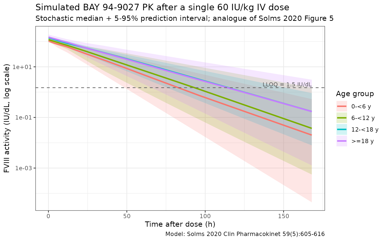
Typical CL and Vc back-check
Solms 2020 Table 2 reports, for the reference patient (LBW = 49.1 kg, VWF = 110 IU/dL), CL = 1.09 dL/h and Vc = 26.2 dL. Reproducing those numbers from the typical-value simulation is the simplest possible self-consistency check.
ev_ref <- rxode2::et(amt = 60 * 70, time = 0, cmt = "central") |>
  rxode2::et(seq(0, 0))
sim_ref <- rxode2::rxSolve(
  mod_typ, events = ev_ref,
  params = data.frame(LBM = 49.1, VWF = 110),
  returnType = "data.frame"
)
#> ℹ omega/sigma items treated as zero: 'etalcl', 'etalvc'

ref_pars <- sim_ref[1, c("cl", "vc"), drop = FALSE]
ref_pars$kel        <- ref_pars$cl / ref_pars$vc
ref_pars$thalf      <- log(2) / ref_pars$kel

knitr::kable(
  ref_pars,
  caption = paste0("Typical-value PK parameters at the reference 49.1 kg LBW",
                   " and 110 IU/dL VWF."),
  digits  = c(3, 2, 4, 2)
)| cl | vc | kel | thalf |
|---|---|---|---|
| 1.09 | 26.2 | 0.0416 | 16.66 |
The model returns CL = 1.09 dL/h and Vc = 26.2 dL, with terminal half-life t_half = 16.7 h – matching the values reported in Solms 2020 Table 2 (CL = 1.09 dL/h, Vc = 26.2 dL) and consistent with the median t_half of 17.4 h reported for adults in Solms 2020 Table 3.
PKNCA validation
Use PKNCA to compute Cmax, AUC0-inf, and terminal half-life by age group, and compare against Solms 2020 Table 3, which reports geometric mean (geometric % CV) PK parameters from empirical Bayes individual estimates after a 60 IU/kg dose.
sim_nca <- sim |>
  filter(!is.na(Cc)) |>
  select(id, time, Cc, age_group)

# Guarantee a time=0 row per (id, age_group) so PKNCA can anchor AUC0-*.
# IV dose with no absorption: pre-dose Cc=0 in severe haemophilia A is
# the correct biological value (FVIII < 1 IU/dL by inclusion criterion;
# treated here as 0).
sim_nca <- dplyr::bind_rows(
  sim_nca,
  sim_nca |> dplyr::distinct(id, age_group) |>
    dplyr::mutate(time = 0, Cc = 0)
) |>
  dplyr::distinct(id, age_group, time, .keep_all = TRUE) |>
  dplyr::arrange(id, age_group, time)

dose_df <- events |>
  filter(EVID == 1) |>
  transmute(id = ID, time = TIME, amt = AMT, age_group, WT)

conc_obj <- PKNCA::PKNCAconc(sim_nca, Cc ~ time | age_group + id,
                             concu = "IU/dL",
                             timeu = "h")
dose_obj <- PKNCA::PKNCAdose(dose_df, amt ~ time | age_group + id,
                             doseu = "IU")

intervals <- data.frame(
  start      = 0,
  end        = Inf,
  cmax       = TRUE,
  tmax       = TRUE,
  aucinf.obs = TRUE,
  half.life  = TRUE,
  clast.obs  = TRUE,
  lambda.z   = TRUE
)

nca_res <- PKNCA::pk.nca(PKNCA::PKNCAdata(conc_obj, dose_obj,
                                          intervals = intervals))
nca_tbl <- as.data.frame(nca_res$result)

geo_mean   <- function(x) exp(mean(log(x[x > 0]), na.rm = TRUE))
geo_cv_pct <- function(x) {
  s <- stats::sd(log(x[x > 0]), na.rm = TRUE)
  100 * sqrt(exp(s^2) - 1)
}

per_subject <- sim |>
  group_by(id, age_group) |>
  summarise(
    WT  = first(WT),
    LBM = first(LBM),
    Vc  = first(vc),
    .groups = "drop"
  )

auc_per_subject <- nca_tbl |>
  filter(PPTESTCD == "aucinf.obs") |>
  transmute(id, age_group, AUC = PPORRES)

thalf_per_subject <- nca_tbl |>
  filter(PPTESTCD == "half.life") |>
  transmute(id, age_group, thalf = PPORRES)

combined <- per_subject |>
  left_join(auc_per_subject, by = c("id", "age_group")) |>
  left_join(thalf_per_subject, by = c("id", "age_group")) |>
  mutate(
    # Paper's Table 3 reports AUCstand at the 60 IU/kg dose in IU*h/dL --
    # the absolute simulated AUC0-inf (not per-kg) is what should match.
    auc          = AUC,
    CL_per_kg    = 60 / AUC,             # = dose_per_kg / AUC; one-compartment IV  =>  CL/WT
    Vss_per_kg   = Vc / WT
  )

cl_vss_summary <- combined |>
  group_by(age_group) |>
  summarise(
    n              = sum(!is.na(AUC)),
    auc_geo_mean   = geo_mean(auc),
    auc_geo_cv     = geo_cv_pct(auc),
    thalf_geo_mean = geo_mean(thalf),
    thalf_geo_cv   = geo_cv_pct(thalf),
    cl_geo_mean    = geo_mean(CL_per_kg),
    cl_geo_cv      = geo_cv_pct(CL_per_kg),
    vss_geo_mean   = geo_mean(Vss_per_kg),
    vss_geo_cv     = geo_cv_pct(Vss_per_kg),
    .groups        = "drop"
  )

knitr::kable(
  cl_vss_summary,
  caption = paste0("Simulated geometric-mean PK parameters by age group ",
                   "after a single 60 IU/kg IV BAY 94-9027 dose."),
  digits  = c(0, 0, 0, 1, 1, 1, 4, 1, 3, 1)
)| age_group | n | auc_geo_mean | auc_geo_cv | thalf_geo_mean | thalf_geo_cv | cl_geo_mean | cl_geo_cv | vss_geo_mean | vss_geo_cv |
|---|---|---|---|---|---|---|---|---|---|
| 0-<6 y | 25 | 2137 | 42.1 | 13.5 | 39.4 | 0.0281 | 42.1 | 0.545 | 13.7 |
| 6-<12 y | 28 | 2662 | 39.0 | 15.4 | 36.6 | 0.0225 | 39.0 | 0.499 | 15.7 |
| 12-<18 y | 12 | 3368 | 26.1 | 16.9 | 27.0 | 0.0178 | 26.1 | 0.434 | 11.2 |
| >=18 y | 133 | 3694 | 37.6 | 17.1 | 33.4 | 0.0162 | 37.6 | 0.400 | 15.5 |
Comparison against Solms 2020 Table 3
Solms 2020 Table 3 reports geometric mean (geometric % CV) AUC_stand, t_half, weight-normalized CL, and weight-normalized Vss after a 60 IU/kg dose, in four age bands. Differences > 20% from the published geometric means would indicate a coding problem.
published <- tibble::tribble(
  ~age_group,   ~published_auc,  ~published_auc_cv,
  ~published_thalf, ~published_thalf_cv,
  ~published_cl,   ~published_cl_cv,
  ~published_vss,  ~published_vss_cv,
  "0-<6 y",     2159, 27.3, 13.1, 21.0, 0.0278, 27.3, 0.524, 11.6,
  "6-<12 y",    2717, 22.4, 15.1, 19.4, 0.0221, 22.4, 0.481, 14.5,
  "12-<18 y",   3441, 34.2, 16.8, 25.2, 0.0174, 34.2, 0.423, 15.5,
  ">=18 y",     4052, 31.1, 17.4, 28.8, 0.0148, 31.1, 0.373, 15.6
) |>
  mutate(age_group = factor(age_group,
                            levels = c("0-<6 y", "6-<12 y",
                                       "12-<18 y", ">=18 y")))

comparison <- published |>
  left_join(cl_vss_summary |>
              select(age_group,
                     simulated_auc   = auc_geo_mean,
                     simulated_thalf = thalf_geo_mean,
                     simulated_cl    = cl_geo_mean,
                     simulated_vss   = vss_geo_mean),
            by = "age_group") |>
  mutate(
    auc_pct_diff   = round(100 * (simulated_auc   - published_auc)   /
                             published_auc, 1),
    thalf_pct_diff = round(100 * (simulated_thalf - published_thalf) /
                             published_thalf, 1),
    cl_pct_diff    = round(100 * (simulated_cl    - published_cl)    /
                             published_cl, 1),
    vss_pct_diff   = round(100 * (simulated_vss   - published_vss)   /
                             published_vss, 1)
  )

knitr::kable(
  comparison,
  caption = paste0("Simulated vs. Solms 2020 Table 3 PK parameters by age ",
                   "group at a single 60 IU/kg dose. AUC = AUC0-inf in ",
                   "IU*h/dL. CL = weight-normalized clearance in ",
                   "dL/(h*kg). Vss = weight-normalized steady-state volume ",
                   "in dL/kg. t_half = terminal half-life in h."),
  digits  = c(0, 0, 1, 1, 1, 4, 1, 3, 1, 0, 1, 4, 3, 1, 1, 1, 1)
)| age_group | published_auc | published_auc_cv | published_thalf | published_thalf_cv | published_cl | published_cl_cv | published_vss | published_vss_cv | simulated_auc | simulated_thalf | simulated_cl | simulated_vss | auc_pct_diff | thalf_pct_diff | cl_pct_diff | vss_pct_diff |
|---|---|---|---|---|---|---|---|---|---|---|---|---|---|---|---|---|
| 0-<6 y | 2159 | 27.3 | 13.1 | 21.0 | 0.0278 | 27.3 | 0.524 | 11.6 | 2137 | 13.5 | 0.0281 | 0.545 | -1.0 | 2.7 | 1.0 | 4.0 |
| 6-<12 y | 2717 | 22.4 | 15.1 | 19.4 | 0.0221 | 22.4 | 0.481 | 14.5 | 2662 | 15.4 | 0.0225 | 0.499 | -2.0 | 1.7 | 2.0 | 3.8 |
| 12-<18 y | 3441 | 34.2 | 16.8 | 25.2 | 0.0174 | 34.2 | 0.423 | 15.5 | 3368 | 16.9 | 0.0178 | 0.434 | -2.1 | 0.5 | 2.4 | 2.6 |
| >=18 y | 4052 | 31.1 | 17.4 | 28.8 | 0.0148 | 31.1 | 0.373 | 15.6 | 3694 | 17.1 | 0.0162 | 0.400 | -8.8 | -1.8 | 9.7 | 7.4 |
Errata
No published erratum was located for Solms 2020 (Clin Pharmacokinet
2020;59(5):605-616) via PubMed (esearch on PMID 31749076 with the
erratum publication type filter), Crossref (no update-to
relations on doi:10.1007/s40262-019-00832-7), or the journal landing
page. The packaged parameter values are taken from Solms 2020 Table 2,
“Chromogenic assay” column, and the equations stated in the Methods
section (Section 2.2) and the Table 2 footnotes. The reference LBW of
49.1 kg matches the value used in the Table 2 footnote equations and is
slightly different from the cohort median LBW of 49.4 kg reported in
Table 1; the 49.1 kg value is preserved here as the centering reference
because that is what the fitted model uses.
Assumptions and deviations
-
Lean body weight (LBW) covariate stored as canonical
LBM. Solms 2020 uses the column nameLBW(lean body weight); the canonical column ininst/references/covariate-columns.mdisLBM(lean body mass). LBW and LBM refer to the same biological quantity (total body weight minus body fat); only the abbreviation differs by literature convention. ThecovariateDataentry in the model file recordssource_name = "LBW", matching the precedent set byGarmann_2017_BAY81_8973(same author group, same drug class). -
LBW reference 49.1 kg vs. cohort median 49.4 kg.
Solms 2020 Table 1 reports the cohort median LBW as 49.4 kg (range
10-75); the Table 2 footnote equations centre LBW at 49.1 kg. The 0.3 kg
discrepancy appears in the published paper itself and is preserved in
the packaged model – the centering value 49.1 kg is what the fitted CL
and Vc estimates are conditioned on, so changing it would change the
typical values reported in Table 2. Downstream users should pass
LBMin kg using the same definition the source dataset used (lean body mass via the Hume / James / FFM convention of their choice). -
LBW body-composition formula not specified. Solms
2020 does not state the formula used to compute LBW from anthropometric
measurements. In haemophilia popPK literature LBW is most commonly
computed via the Hume
- or James (1976) formula. The vignette’s virtual cohort uses a
male-specific James approximation
LBW = 1.10 * WT - 128 * (WT / HT_m)^2purely to populate the covariate column for simulation; it does not prescribe a specific formula for downstream users.
- or James (1976) formula. The vignette’s virtual cohort uses a
male-specific James approximation
- VWF treated as time-fixed. Solms 2020 uses VWF measured at baseline as the covariate for CL; within-subject VWF time course is not characterized. The vignette samples VWF once per virtual subject from a log-normal centered at the cohort median 110 IU/dL (mean 122, SD 55.3) and treats it as time-fixed throughout the dosing interval.
- VWF in paediatric subjects. VWF measurements were not available in PROTECT VIII Kids; the CL-VWF relationship is informed by adult and adolescent data only. Solms 2020 argues (Discussion) that the adult/adolescent VWF range (47-366 IU/dL) covers the paediatric range typically observed in the literature, so the relationship is expected to extend. The virtual cohort samples VWF identically across all four age bands.
- One-compartment selected over two-compartment. A two-compartment model was tested during base-model development; the peripheral compartment could not be identified (intercompartmental CL RSE > 70%) and the one-compartment goodness-of-fit showed no trend. The packaged model is the published one-compartment final model (Solms 2020 Figure 2).
- No inter-occasion variability (IOV). Solms 2020 estimated IOV (variance 0.0195 for CL and 0.00475 for Vc; base-model section) but did not retain it in the final model because inclusion had no effect on the population estimates of CL or Vc. The packaged model has no IOV; downstream users who want to assess the impact of IOV can add it via the rxode2 event table OCC column with externally-supplied variance estimates.
- One-stage assay parameters not implemented. Solms 2020 Table 2 also reports the same final model refit to the one-stage assay subset (1648 observations from 146 subjects in phase I and PROTECT VIII). Those parameters are similar but not identical to the chromogenic-assay parameters (CL 1.02 vs. 1.09 dL/h, Vc 24.2 vs. 26.2 dL, e_lbw_cl 0.858 vs. 0.707, e_lbw_vc 0.683 vs. 0.887, etc.). The packaged model uses the chromogenic-assay values, since that is the primary final model and was used for the simulation analyses (Tables 3, 4, 5).
-
Combined RUV interpreted as
C * (1 + e1) + e2. Solms 2020 Methods 2.2 states that the residual error is “a so-called combined error model consisting of a concentration-proportional and a concentration-independent additive part”. The packaged model usesCc ~ add(addSd) + prop(propSd), which implements exactly this form in nlmixr2. The reported variances (additive 1.78, proportional 0.175) are converted to SDs (addSd = sqrt(1.78) = 1.3342 IU/dL; propSd = sqrt(0.175) = 0.4183, matching the 41.8% CV reported in Table 2 footnote d). -
No baseline FVIII offset. The chromogenic assay
measures total FVIII activity, but in severe haemophilia A baseline
endogenous FVIII activity is by definition < 1 IU/dL (the inclusion
criterion). The packaged model treats simulated
Ccas the activity attributable to BAY 94-9027 above this near-zero baseline. -
Infusion duration handled at the event-table level.
BAY 94-9027 is given as an IV infusion. The packaged model is agnostic
to infusion duration; users supply an
RATE(or duration) column in their event table to model the infusion shape if needed. The vignette’s simulations use an instantaneous bolus, which is a reasonable approximation for a short IV infusion when judging trough activity but slightly overestimates very-early Cmax. - No anti-PEG-antibody handling. Solms 2020 excluded seven patients with anti-PEG antibodies and/or perceived loss of efficacy from the final model. The packaged model is the post-exclusion model and does not carry any anti-PEG covariate; users analysing real-world post-marketing data should be aware that anti-PEG antibody status is a known modifier of PEGylated FVIII exposure in some patients.
- Virtual cohort. Per-band sample sizes (n = 25, 28, 12, 133) match the Solms 2020 Table 3 sample sizes for the per-band PK summary. Body weight and height within each band were simulated from log-normal distributions tuned to span typical paediatric / adolescent / adult ranges; LBW was derived from a male James (1976) approximation. VWF was sampled from a log-normal centred at the cohort median 110 IU/dL with the observed CV. Joint covariate structure (e.g., narrow weight range within each paediatric age year, or actual within-trial VWF-age correlation) is not simulated.