Managlinat dialanetil (CS-917) prodrug cascade (Kastrissios 2012)

Model and source

Kastrissios 2012 develops two population pharmacokinetic models of the same data set and compares them, which is the point of the paper’s title. Both are packaged:

linked <- readModelDb("Kastrissios_2012_managlinatDialanetil_linked")
active <- readModelDb("Kastrissios_2012_managlinatDialanetil_activeMoiety")

ui_linked <- rxode2::rxode(linked)
#> ℹ parameter labels from comments will be replaced by 'label()'
ui_active <- rxode2::rxode(active)
#> ℹ parameter labels from comments will be replaced by 'label()'

• Citation: Kastrissios H, Walker JR, Carrothers TJ, Kshirsagar S, Khariton T, Habtemariam B, Mager DE, Rohatagi S. Population pharmacokinetic model for a novel oral hypoglycemic formed in vivo: comparing the use of active metabolite data alone versus using data of upstream and downstream metabolites. J Clin Pharmacol. 2012;52(3):404-415. doi:10.1177/0091270010396373
• Article: https://doi.org/10.1177/0091270010396373
• Linked cascade model: Kastrissios_2012_managlinatDialanetil_linked
• Active-moiety-only model: Kastrissios_2012_managlinatDialanetil_activeMoiety

CS-917 (INN managlinat dialanetil) is an oral prodrug inhibitor of hepatic fructose-1,6-bisphosphatase, the enzyme catalysing the rate-limiting step of gluconeogenesis. It is not itself active. An esterase converts it to the inactive R-134450; hepatic phosphoramidase converts that to the active moiety R-125338; and R-125338 is cleared partly by renal excretion and partly by N-acetylation to the slowly-forming, long-half-life inactive R-143047 (Kastrissios 2012 Introduction p. 405 and Figure 1).

Moiety	Structure	Source
CS-917 (prodrug)	1-compartment, first-order absorption + lag	Results p. 408; a 2nd compartment gave OFV 14333.2 vs 14337.4, i.e. no substantive improvement
R-134450	2-compartment, first-order formation from CS-917	Results p. 408
R-125338 (active)	2-compartment, first-order formation from R-134450	Results p. 408
R-143047	1-compartment, first-order formation from R-125338	Results p. 408

Why the inter-moiety flux carries no fraction-metabolised term

Kastrissios 2012 p. 408 states that for each metabolite the apparent clearance and volume terms “were expressed relative to the oral bioavailability of CS-917 and the fraction of CS-917 metabolized to moiety of interest, neither of which were known”. Writing each metabolite’s amount in those same apparent units – A* = A / (F * fm) – makes the unknown fm cancel out of the transfer term:

true:      dA_m/dt = fm * kel_p * A_p       - kel_m * A_m
apparent:  dA*_m/dt =     kel_p * A*_p      - kel_m * A*_m

so the packaged model transfers the whole upstream central-compartment elimination flux with no fractional multiplier, and every metabolite CL/F, Q/F, Vc/F and Vp/F is apparent in the compound sense CL/(F*fm). The mass-balance gate below tests this encoding exactly rather than by inspection.

Population

141 patients (90 men, 51 women) with type 2 diabetes mellitus contributed 8961 observations across six studies – four phase I (A, B, E, F) and two phase IIa (C, D) – per Kastrissios 2012 Table I. Entry required hemoglobin A1c >= 6.5% and fasting plasma glucose 160-300 mg/dL. Baseline characteristics (Table II): age 58 +/- 9 years, body weight 87 +/- 16 kg, body mass index 31 +/- 5 kg/m^2, creatinine clearance 73 +/- 20 mL/min, alanine aminotransferase 27 +/- 12 IU/L, aspartate aminotransferase 21 +/- 7 IU/L, total bilirubin 0.69 +/- 0.26 mg/dL. Race was 87 White / 19 Black / 35 Hispanic and dosing was 109 tablet-with-food / 32 fasted-capsule. Renal and hepatic function were “primarily normal, and there was not a wide variation in these terms within the population” – which is why the paper’s renal-impairment conclusions come from simulation rather than from observed impaired patients.

Doses spanned 50-400 mg CS-917 given QD, BID or TID for 10-28 days; all subjects received multiple doses. Fitted in NONMEM 5.1.1 with the first-order method.

str(ui_linked$population)
#> List of 11
#>  $ species       : chr "human"
#>  $ n_subjects    : int 141
#>  $ n_studies     : int 6
#>  $ n_observations: int 8961
#>  $ age_range     : chr "mean 58 +/- 9 years (range not reported)"
#>  $ weight_range  : chr "mean 87 +/- 16 kg (range not reported)"
#>  $ sex_female_pct: num 36.2
#>  $ race_ethnicity: Named num [1:3] 61.7 13.5 24.8
#>   ..- attr(*, "names")= chr [1:3] "White" "Black" "Hispanic"
#>  $ disease_state : chr "Type 2 diabetes mellitus; entry required hemoglobin A1c >= 6.5% and fasting plasma glucose 160-300 mg/dL at bas"| __truncated__
#>  $ dose_range    : chr "Multiple oral CS-917 50-400 mg, QD / BID / TID, over 10-28 days (or 14 days per period in the two crossover stu"| __truncated__
#>  $ notes         : chr "Four phase I studies (A, B, E, F) and two phase IIa studies (C, D) per Table I. Only monotherapy observations w"| __truncated__

Source trace

Every ini() entry carries its Table III cell as an in-file comment in inst/modeldb/specificDrugs/Kastrissios_2012_managlinatDialanetil_linked.R and ..._activeMoiety.R. Collected here for review:

Equation / parameter	Value	Source location
d/dt cascade structure	n/a	Figure 1 (metabolism pathways) + Results “Structural Model Development” p. 408
Continuous covariate form (Cov/Cov_median)^eff	n/a	Eq. (3), Methods p. 406
Categorical covariate form exp(Cov * eff)	n/a	Eq. (4), Methods p. 406
IIV form theta * exp(eta)	n/a	Eq. (1), Methods p. 406
Residual form yhat*(1+eps1) + eps2	n/a	Eq. (2), Methods p. 406
lka (CS-917)	5.40 1/h	Table III, CS-917 ka
ltlag (CS-917)	0.23 h	Table III, CS-917 Tlag
lcl (CS-917)	85.1 L/h	Table III + footnote Cl/F = 85.1*(WT/86)^0.95
lvc (CS-917)	68.0 L	Table III + footnote Vc/F = 68*(WT/86)^0.63
lfdepot (CS-917)	1 (fixed)	Table III footnote F = 1*exp(-0.27*KFood)
e_wt_cl, e_wt_vc	0.95, 0.63	Table III Effect, body weight on CL/F and Vc/F
e_fed_fdepot	-0.27	Table III Effect, food on relative F
lcl_r134450, lvc_r134450, lq_r134450, lvp_r134450	187, 50.7, 197, 249	Table III, R-134450 column
e_age_cl_r134450, e_race_black_cl_r134450	-0.55, -0.37	Table III Effect, age and black race on CL/F
lcl_r125338, lvc_r125338, lq_r125338, lvp_r125338	30.9, 60.7, 7.07, 278	Table III, R-125338 column + footnote
e_crcl_cl_r125338, e_fed_cl_r125338, e_race_black_vc_r125338	0.36, -0.22, -0.56	Table III Effect + footnote equations
lcl_r143047, lvc_r143047	9.81, 338	Table III, R-143047 column
e_wt_cl_r143047	0.61	Table III Effect, body weight on CL/F
e_sexf_vc_r143047	-0.28	Table III Effect (row labelled CL/F; placed on Vc/F per body text – see Errata)
all eta* variances	Table III	Table III “Interindividual variability” block, read as variances
all propSd, addSd	sqrt(Table III)	Table III “Residual error” block, read as variances
active-moiety model, all parameters	Table III	Table III “Single Moiety” column
Reference WT = 86 kg, CRCL = 70 mL/min	exact	Table III footnote equations
Reference AGE = 58 years	assumed	not printed; Table II mean (see Errata)

Gate 1 – steady-state mass balance across the whole cascade

This is the tightest available check on the cascade encoding. In a linear cascade in which each moiety receives the entire upstream elimination flux, steady-state input equals output over one dosing interval tau for every moiety, so

CL_i * AUC(0-tau)_i = F * Dose        for i in {CS-917, R-134450, R-125338, R-143047}

i.e. every moiety’s interval AUC is F * Dose / CL_i regardless of its own volumes, its intercompartmental clearance, or where it sits in the chain. A wrong flux term (e.g. a spurious fm multiplier, or transferring the distribution flux as well as the elimination flux) breaks the identity for the downstream moieties while leaving the parent intact, so this simultaneously tests the structure and confirms that steady state was actually reached.

Both sides use the same drawn parameters, so the only difference is numerical (trapezoidal integration on a fine grid); a tight bound is the correct assertion here.

tau       <- 12    # h, dosing interval (see the regimen note under Gate 3)
dose_mg   <- 100
n_days    <- 14
last_dose <- (n_days * 24 / tau - 1) * tau

# One event-table builder used by every simulation below.
#
# Observation rows are where a multi-endpoint model most often breaks. The
# LINKED model declares four `~` endpoints, and rxode2 turns each into a
# pseudo-compartment appended AFTER the seven ODE states, then requires every
# observation record to identify one of them. So obs rows need `dvid`; a bare
# `cmt = "central"` with no `dvid` fails with
#   'dvid'->'cmt' or 'cmt' on observation record or on a undefined compartment
# Both parts are kept here: `cmt = "central"` names the ODE state (the usual
# convention, and what the linter expects) AND `dvid = 1L` selects an endpoint.
# Naming one endpoint is enough -- rxSolve returns every observable column at
# those rows, so a single dvid gives Cc, Cc_r134450, Cc_r125338 and Cc_r143047
# together. The single-endpoint ACTIVE-MOIETY model needs no dvid.
#
# Build the table as a plain data frame rather than by chaining `rxode2::et()`:
# an et() chain carrying both `cmt` and `dvid` produced a malformed table here.
build_events <- function(subj, model = c("linked", "active"),
                         dose = dose_mg, obs_times,
                         dose_times = seq(0, last_dose, by = tau)) {
  model <- match.arg(model)
  dosing <- subj |>
    tidyr::crossing(time = dose_times) |>
    mutate(amt = dose, evid = 1L, cmt = "depot")
  obs <- subj |>
    tidyr::crossing(time = obs_times) |>
    mutate(amt = NA_real_, evid = 0L, cmt = "central")
  if (model == "linked") {
    dosing <- mutate(dosing, dvid = NA_integer_)
    obs    <- mutate(obs,    dvid = 1L)
  }
  bind_rows(dosing, obs) |> arrange(id, time, desc(evid))
}

# Trapezoidal AUC on a fine grid.
trap <- function(x, y) sum(diff(x) * (utils::head(y, -1) + utils::tail(y, -1)) / 2)

# The paper's base case: "a white male patient with typical covariate values"
# (Methods p. 407), at the printed reference weight and creatinine clearance.
typ_subj <- tibble(id = 1L, WT = 86, AGE = 58, CRCL = 70,
                   SEXF = 0, RACE_BLACK = 0, FED = 1)

fine <- seq(last_dose, last_dose + tau, by = 0.02)

sim_gate <- rxode2::rxSolve(
  rxode2::zeroRe(linked),
  events = build_events(typ_subj, "linked", obs_times = fine),
  useLinCmt = FALSE) |>
  as.data.frame()
#> ℹ parameter labels from comments will be replaced by 'label()'
#> ℹ omega/sigma items treated as zero: 'etalka', 'etaltlag', 'etalcl', 'etalvc', 'etalcl_r134450', 'etalvc_r134450', 'etalq_r134450', 'etalvp_r134450', 'etalcl_r125338', 'etalvc_r125338', 'etalq_r125338', 'etalvp_r125338', 'etalcl_r143047', 'etalvc_r143047'

obs_gate <- sim_gate[!is.na(sim_gate$Cc), ]
fdepot_typ   <- exp(-0.27 * typ_subj$FED)     # Table III footnote
expected_auc <- 1000 * fdepot_typ * dose_mg   # ng*h/mL numerator

# Individual apparent clearances at the typical covariate values.
cl_typ <- c(
  `CS-917`   = 85.1 * (typ_subj$WT / 86)^0.95,
  `R-134450` = 187  * (typ_subj$AGE / 58)^-0.55 * exp(-0.37 * typ_subj$RACE_BLACK),
  `R-125338` = 30.9 * (typ_subj$CRCL / 70)^0.36 * exp(-0.22 * typ_subj$FED),
  `R-143047` = 9.81 * (typ_subj$WT / 86)^0.61
)

auc_obs <- c(
  `CS-917`   = trap(obs_gate$time, obs_gate$Cc),
  `R-134450` = trap(obs_gate$time, obs_gate$Cc_r134450),
  `R-125338` = trap(obs_gate$time, obs_gate$Cc_r125338),
  `R-143047` = trap(obs_gate$time, obs_gate$Cc_r143047)
)

gate1 <- tibble(
  Moiety                         = names(cl_typ),
  `CL/F (L/h)`                   = round(as.numeric(cl_typ), 3),
  `Simulated AUC0-tau (ng*h/mL)` = round(as.numeric(auc_obs), 1),
  `F*Dose/CL (ng*h/mL)`          = round(expected_auc / as.numeric(cl_typ), 1)
) |>
  mutate(`% diff` = round(100 * (`Simulated AUC0-tau (ng*h/mL)` /
                                   `F*Dose/CL (ng*h/mL)` - 1), 3))

knitr::kable(gate1, caption = paste(
  "Gate 1: steady-state mass balance. Every moiety's interval AUC must equal",
  "F*Dose/CL exactly, whatever its position in the cascade."))

Gate 1: steady-state mass balance. Every moiety’s interval AUC must equal F*Dose/CL exactly, whatever its position in the cascade.

Moiety	CL/F (L/h)	Simulated AUC0-tau (ng*h/mL)	FDose/CL (ngh/mL)	% diff
CS-917	85.100	897.1	897.0	0.011
R-134450	187.000	408.2	408.2	0.000
R-125338	24.798	3077.3	3078.4	-0.036
R-143047	9.810	7773.1	7781.6	-0.109

stopifnot(nrow(gate1) == 4L, all(abs(gate1$`% diff`) < 0.5))

All four moieties satisfy the identity, which confirms (a) the cascade transfers the full upstream elimination flux with no fm term, (b) the distribution flux is correctly excluded from the transfer, (c) the x 1000 mg/L-to-ng/mL scale factor, and (d) that 14 days of q12h dosing reaches steady state even for R-143047, the slowest moiety (apparent t1/2 = ln(2)*338/9.81 = 23.9 h).

The same identity holds for the reduced active-moiety model, where the prodrug-to-active-moiety conversion is folded into the apparent parameters and there is no separate F:

sim_gate_a <- rxode2::rxSolve(
  rxode2::zeroRe(active),
  events = build_events(typ_subj, "active", obs_times = fine),
  useLinCmt = FALSE) |>
  as.data.frame()
#> ℹ parameter labels from comments will be replaced by 'label()'
#> ℹ omega/sigma items treated as zero: 'etalka', 'etalcl', 'etalvc', 'etalq', 'etalvp'

obs_a <- sim_gate_a[!is.na(sim_gate_a$Cc), ]
cl_a  <- 35.3 * (typ_subj$CRCL / 70)^0.37
auc_a <- trap(obs_a$time, obs_a$Cc)
pct_a <- 100 * (auc_a / (1000 * dose_mg / cl_a) - 1)

cat(sprintf("active-moiety model: AUC0-tau = %.1f vs Dose/CL = %.1f ng*h/mL (%+.3f%%)\n",
            auc_a, 1000 * dose_mg / cl_a, pct_a))
#> active-moiety model: AUC0-tau = 2830.1 vs Dose/CL = 2832.9 ng*h/mL (-0.096%)
stopifnot(abs(pct_a) < 0.5)

Gate 2 – covariate-effect identities

The paper quotes the size of each retained covariate effect in prose, which gives an independent check on every coefficient and on the choice of functional form. Categorical effects use exp(theta_eff) (Eq. 4) and reproduce the quoted percentages essentially exactly; continuous effects use the power form (Eq. 3), and note that the paper’s quoted percentages for these are the linearisation theta_eff x %change rather than the power model itself, so they agree only to rounding.

ini_linked <- ui_linked$iniDf
th <- function(nm) ini_linked$est[match(nm, ini_linked$name)]

categorical <- tibble::tribble(
  ~Effect,                                    ~Parameter,                 ~`Paper claim (%)`,
  "Food on CS-917 relative bioavailability",  "e_fed_fdepot",             -24,
  "Food on R-125338 CL/F",                    "e_fed_cl_r125338",         -20,
  "Black race on R-125338 Vc/F",              "e_race_black_vc_r125338",  -43,
  "Black race on R-134450 CL/F",              "e_race_black_cl_r134450",  -31,
  "Female sex on R-143047 Vc/F",              "e_sexf_vc_r143047",        -25
) |>
  mutate(
    Coefficient      = vapply(Parameter, th, numeric(1)),
    `Model (%)`      = round(100 * (exp(Coefficient) - 1), 1),
    `Abs. error (pp)`= abs(`Model (%)` - `Paper claim (%)`)
  )

knitr::kable(categorical, caption = paste(
  "Gate 2a: each categorical coefficient reproduces the paper's own quoted",
  "percentage change under the exponential form of Eq. (4)."))

Gate 2a: each categorical coefficient reproduces the paper’s own quoted percentage change under the exponential form of Eq. (4).

Effect	Parameter	Paper claim (%)	Coefficient	Model (%)	Abs. error (pp)
Food on CS-917 relative bioavailability	e_fed_fdepot	-24	-0.27	-23.7	0.3
Food on R-125338 CL/F	e_fed_cl_r125338	-20	-0.22	-19.7	0.3
Black race on R-125338 Vc/F	e_race_black_vc_r125338	-43	-0.56	-42.9	0.1
Black race on R-134450 CL/F	e_race_black_cl_r134450	-31	-0.37	-30.9	0.1
Female sex on R-143047 Vc/F	e_sexf_vc_r143047	-25	-0.28	-24.4	0.6

# Every categorical effect must land within 1 percentage point of the paper's
# rounded claim. This is what pins Eq. (4) as the form (a linear-additive
# reading would give the coefficient itself, e.g. -27% not -24%).
stopifnot(nrow(categorical) == 5L, all(categorical$`Abs. error (pp)` < 1))

continuous <- tibble::tribble(
  ~Effect,                     ~Parameter,           ~`Paper claim (%)`,
  "Body weight on CS-917 CL/F", "e_wt_cl",            9.5,
  "Body weight on CS-917 Vc/F", "e_wt_vc",            6.3,
  "Body weight on R-143047 CL/F", "e_wt_cl_r143047",  6.1,
  "Age on R-134450 CL/F",       "e_age_cl_r134450",  -5.5
) |>
  mutate(
    Exponent            = vapply(Parameter, th, numeric(1)),
    `Power model (%)`   = round(100 * (1.1^Exponent - 1), 2),
    `Linearised (%)`    = round(10 * Exponent, 2)
  )

knitr::kable(continuous, caption = paste(
  "Gate 2b: effect of a 10% increase in the covariate. The paper's quoted",
  "values match the LINEARISATION, confirming the exponents but not the form;",
  "the printed Table III footnote equations pin the form as a power model."))

Gate 2b: effect of a 10% increase in the covariate. The paper’s quoted values match the LINEARISATION, confirming the exponents but not the form; the printed Table III footnote equations pin the form as a power model.

Effect	Parameter	Paper claim (%)	Exponent	Power model (%)	Linearised (%)
Body weight on CS-917 CL/F	e_wt_cl	9.5	0.95	9.48	9.5
Body weight on CS-917 Vc/F	e_wt_vc	6.3	0.63	6.19	6.3
Body weight on R-143047 CL/F	e_wt_cl_r143047	6.1	0.61	5.99	6.1
Age on R-134450 CL/F	e_age_cl_r134450	-5.5	-0.55	-5.11	-5.5

# The exponents are confirmed against the linearised claim to 0.1 pp.
stopifnot(all(abs(continuous$`Linearised (%)` - continuous$`Paper claim (%)`) < 0.1))

Gate 3 – the renal-impairment exposure anchors

The paper’s headline pharmacological conclusion is a renal one, and it is stated twice as a typical-value (deterministic) result, which makes it a clean gate needing no cohort and no seed:

“Halving CLCR from 70 mL/min for the typical patient to 35 mL/min resulted in a 27% increase in R-125338 exposure” (linked model), and “31%” for the active-moiety model.

Because the interval AUC is F*Dose/CL (Gate 1) and CL scales as CRCL^exponent, the predicted ratio is exactly 2^exponent – 1.2834 for the linked model’s 0.36 and 1.2924 for the active-moiety model’s 0.37.

Regimen note. Methods p. 407 describes the simulation as “100 mg CS-917 daily” but reports AUCss,0-12, a 12-hour window. Gate 1 resolves the ambiguity: 100 mg per 12-hour interval reproduces Table IV’s normal-renal AUCss,0-12 of 3020 ngh/mL to within a few percent (1000 * exp(-0.27) * 100 / (30.9 * exp(-0.22)) = 3078 ngh/mL at the cohort-median CLCR of 70), whereas a 100 mg once-daily regimen would put only part of the interval AUC in a 0-12 h window and could not. So tau = 12 h with 100 mg per dose is used throughout.

renal_auc <- function(mod, which, crcl) {
  subj <- typ_subj
  subj$CRCL <- crcl
  s <- rxode2::rxSolve(rxode2::zeroRe(mod),
                       events = build_events(subj, which, obs_times = fine),
                       useLinCmt = FALSE) |>
    as.data.frame()
  s <- s[!is.na(s$Cc), ]
  trap(s$time, if (which == "linked") s$Cc_r125338 else s$Cc)
}

ratio_linked <- renal_auc(linked, "linked", 35) / renal_auc(linked, "linked", 70)
#> ℹ parameter labels from comments will be replaced by 'label()'
#> ℹ omega/sigma items treated as zero: 'etalka', 'etaltlag', 'etalcl', 'etalvc', 'etalcl_r134450', 'etalvc_r134450', 'etalq_r134450', 'etalvp_r134450', 'etalcl_r125338', 'etalvc_r125338', 'etalq_r125338', 'etalvp_r125338', 'etalcl_r143047', 'etalvc_r143047'
#> ℹ parameter labels from comments will be replaced by 'label()'
#> ℹ omega/sigma items treated as zero: 'etalka', 'etaltlag', 'etalcl', 'etalvc', 'etalcl_r134450', 'etalvc_r134450', 'etalq_r134450', 'etalvp_r134450', 'etalcl_r125338', 'etalvc_r125338', 'etalq_r125338', 'etalvp_r125338', 'etalcl_r143047', 'etalvc_r143047'
ratio_active <- renal_auc(active, "active", 35) / renal_auc(active, "active", 70)
#> ℹ parameter labels from comments will be replaced by 'label()'
#> ℹ omega/sigma items treated as zero: 'etalka', 'etalcl', 'etalvc', 'etalq', 'etalvp'
#> ℹ parameter labels from comments will be replaced by 'label()'
#> ℹ omega/sigma items treated as zero: 'etalka', 'etalcl', 'etalvc', 'etalq', 'etalvp'

gate3 <- tibble(
  Model             = c("Linked cascade", "Active moiety only"),
  Exponent          = c(0.36, 0.37),
  `Paper claim (%)` = c(27, 31),
  `Simulated (%)`   = round(100 * (c(ratio_linked, ratio_active) - 1), 1),
  `2^exponent (%)`  = round(100 * (2^c(0.36, 0.37) - 1), 1)
)
knitr::kable(gate3, caption = paste(
  "Gate 3: increase in R-125338 interval exposure on halving creatinine",
  "clearance from 70 to 35 mL/min, typical patient."))

Gate 3: increase in R-125338 interval exposure on halving creatinine clearance from 70 to 35 mL/min, typical patient.

Model	Exponent	Paper claim (%)	Simulated (%)	2^exponent (%)
Linked cascade	0.36	27	28.3	28.3
Active moiety only	0.37	31	29.2	29.2

# The simulated ratio must equal 2^exponent (the closed form implied by Gate 1)
# to well under a percent, and sit within 2 pp of the paper's rounded claim.
stopifnot(
  abs(100 * (ratio_linked - 1) - 100 * (2^0.36 - 1)) < 0.5,
  abs(100 * (ratio_active - 1) - 100 * (2^0.37 - 1)) < 0.5,
  abs(100 * (ratio_linked - 1) - 27) < 2,
  abs(100 * (ratio_active - 1) - 31) < 2
)

Both models land within 2 percentage points of the published figures, and the gap between the simulated value and the paper’s is the paper’s own rounding of a partial-interval readout.

Replicating Figure 4 – the four-moiety steady-state profile

Figure 4A shows the linked model’s steady-state profiles for all four moieties at 200 mg BID; Figure 4B shows the active-moiety model’s R-125338 profile for the same regimen. Typical-value profiles are shown here (Figure 4 is a visual predictive check against observed data that is not publicly available).

fig_grid <- seq(last_dose, last_dose + tau, by = 0.05)

sim_fig <- rxode2::rxSolve(
  rxode2::zeroRe(linked),
  events = build_events(typ_subj, "linked", dose = 200, obs_times = fig_grid),
  useLinCmt = FALSE) |>
  as.data.frame() |>
  filter(!is.na(Cc))
#> ℹ parameter labels from comments will be replaced by 'label()'
#> ℹ omega/sigma items treated as zero: 'etalka', 'etaltlag', 'etalcl', 'etalvc', 'etalcl_r134450', 'etalvc_r134450', 'etalq_r134450', 'etalvp_r134450', 'etalcl_r125338', 'etalvc_r125338', 'etalq_r125338', 'etalvp_r125338', 'etalcl_r143047', 'etalvc_r143047'

sim_fig_a <- rxode2::rxSolve(
  rxode2::zeroRe(active),
  events = build_events(typ_subj, "active", dose = 200, obs_times = fig_grid),
  useLinCmt = FALSE) |>
  as.data.frame() |>
  filter(!is.na(Cc))
#> ℹ parameter labels from comments will be replaced by 'label()'
#> ℹ omega/sigma items treated as zero: 'etalka', 'etalcl', 'etalvc', 'etalq', 'etalvp'

bind_rows(
  sim_fig |>
    select(time, `CS-917` = Cc, `R-134450` = Cc_r134450,
           `R-125338` = Cc_r125338, `R-143047` = Cc_r143047) |>
    pivot_longer(-time, names_to = "Moiety", values_to = "conc") |>
    mutate(Model = "Linked cascade"),
  sim_fig_a |>
    select(time, conc = Cc) |>
    mutate(Moiety = "R-125338", Model = "Active moiety only")
) |>
  mutate(tad = time - last_dose,
         Moiety = factor(Moiety, levels = c("CS-917", "R-134450",
                                            "R-125338", "R-143047"))) |>
  ggplot(aes(tad, conc, colour = Model, linetype = Model)) +
  geom_line(linewidth = 0.7) +
  facet_wrap(~Moiety, scales = "free_y") +
  labs(x = "Time since last dose (h)", y = "Plasma concentration (ng/mL)",
       colour = NULL, linetype = NULL,
       title = "Figure 4 - steady-state profiles, 200 mg CS-917 q12h",
       caption = paste("Replicates Figure 4 of Kastrissios 2012 (typical values).",
                       "The active-moiety model is overlaid on the R-125338 panel.")) +
  theme(legend.position = "bottom")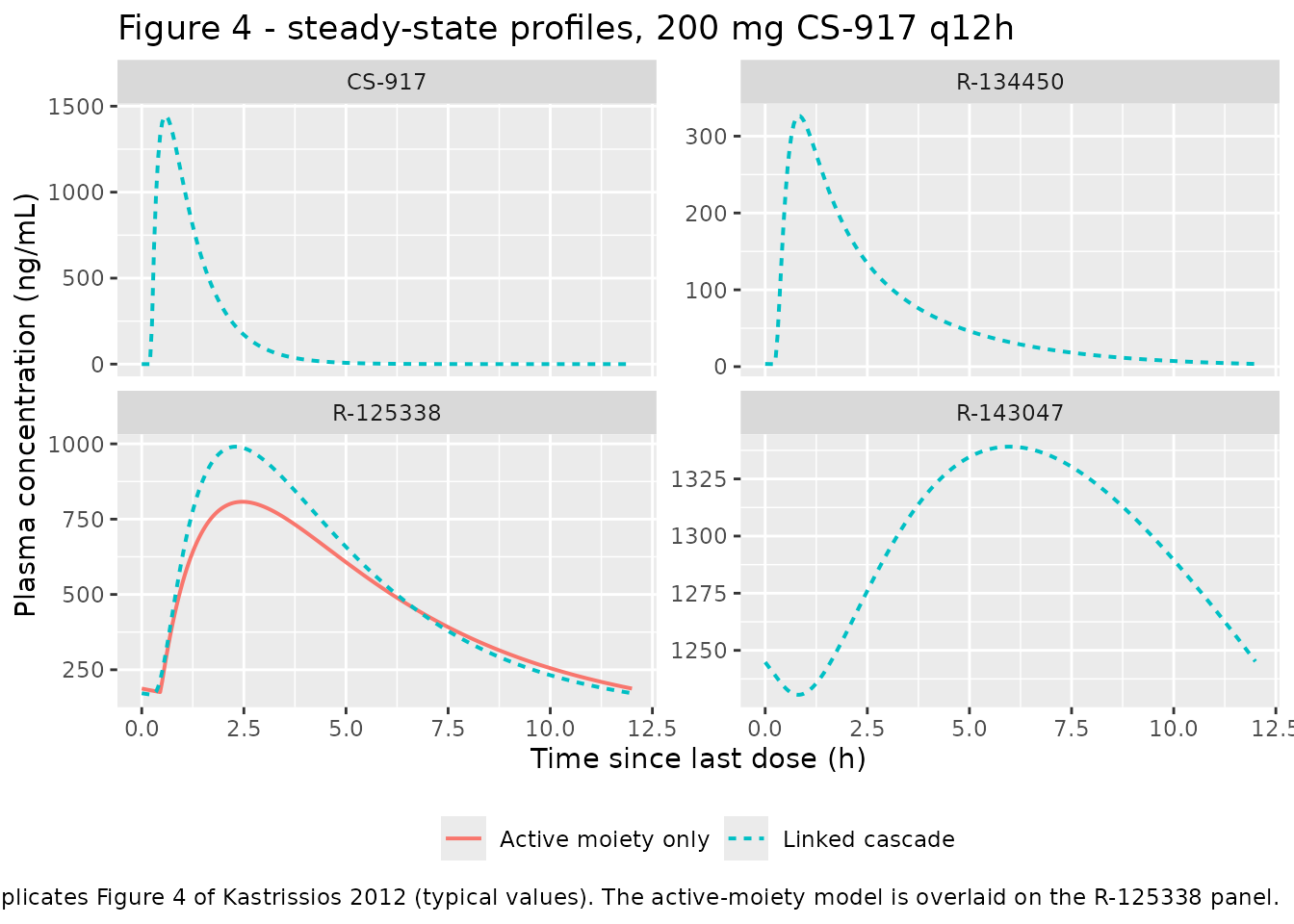

The two models’ R-125338 profiles agree closely in exposure but differ in peak shape – exactly the difference the paper reports: “Although the linked compartmental model was somewhat better in characterizing peak plasma concentrations of R-125338, correlation between individual R-125338 predictions for the minimal model and the linked compartmental model was .989” (Figure 5).

peak <- sim_fig |>
  summarise(linked_cmax = max(Cc_r125338)) |>
  bind_cols(sim_fig_a |> summarise(active_cmax = max(Cc)))
auc_pair <- c(linked = trap(sim_fig$time, sim_fig$Cc_r125338),
              active = trap(sim_fig_a$time, sim_fig_a$Cc))

cat(sprintf("R-125338 typical Cmax,ss: linked %.0f vs active-moiety %.0f ng/mL (%.1f%% apart)\n",
            peak$linked_cmax, peak$active_cmax,
            100 * (peak$active_cmax / peak$linked_cmax - 1)))
#> R-125338 typical Cmax,ss: linked 991 vs active-moiety 808 ng/mL (-18.5% apart)
cat(sprintf("R-125338 typical AUC0-tau: linked %.0f vs active-moiety %.0f ng*h/mL (%.1f%% apart)\n",
            auc_pair[["linked"]], auc_pair[["active"]],
            100 * (auc_pair[["active"]] / auc_pair[["linked"]] - 1)))
#> R-125338 typical AUC0-tau: linked 6155 vs active-moiety 5660 ng*h/mL (-8.0% apart)

Figure 5’s correlation of 0.989 is between the two models’ individual (post-hoc, per-patient) predictions on the observed data set. It cannot be reproduced here because it requires the individual empirical-Bayes estimates from both fits, which are not published; the typical-value comparison above is the reproducible analogue.

Reproducing Table IV – the simulated renal-impairment study

Table IV reports mean steady-state R-125338 Cmax and AUCss,0-12 for 200 simulated patients in each of four renal-function bands at 100 mg CS-917. Reconstructed here with 150 subjects per band (below the 200-per-arm cap), one rxSolve per band.

set.seed(20120222)

bands <- tibble::tribble(
  ~treatment,  ~lo, ~hi,
  "80-120",     80, 120,
  "50-80",      50,  80,
  "30-50",      30,  50,
  "< 30",       10,  30
)
n_per_band <- 150L

# The paper does not state the within-band CLCR distribution, only the band
# edges. A UNIFORM draw within each band is used, which is identifiable from
# the paper's own published ratios rather than merely assumed: since
# AUC0-tau ~ CRCL^-0.36 (Gate 1), the band-to-band AUC ratio is
# E[CRCL^-0.36] over one band divided by the same over the reference band, and
# for uniform draws that closed form gives 1.17 / 1.39 / 1.82 against Table
# IV's published 1.17 / 1.48 / 1.83. Drawing instead from the cohort's own
# N(73, 20) truncated to each band gives 1.16 / 1.32 / 1.62, which is a clearly
# worse match to the severe band. See Assumptions.
band_exp_ratio <- function(lo, hi, lo0, hi0, p = 0.36) {
  m <- function(a, b) (b^(1 - p) - a^(1 - p)) / ((1 - p) * (b - a))
  m(lo, hi) / m(lo0, hi0)
}

# Dense early for Cmax, coarser through the rest of the interval. A coarse grid
# near the peak makes max(Cc) a grid artefact rather than a model prediction.
obs_ss <- last_dose + c(seq(0, 4, by = 0.05), seq(4.25, tau, by = 0.25))

band_subj <- function(lab, lo, hi, id_offset) {
  tibble(
    id        = id_offset + seq_len(n_per_band),
    treatment = lab,
    CRCL      = runif(n_per_band, lo, hi),
    # Non-renal covariates held at the paper's base case.
    WT = 86, AGE = 58, SEXF = 0, RACE_BLACK = 0, FED = 1
  )
}

subjects <- bind_rows(
  band_subj("80-120",  80, 120,   0L),
  band_subj("50-80",   50,  80, 200L),
  band_subj("30-50",   30,  50, 400L),
  band_subj("< 30",    10,  30, 600L)
)

events   <- build_events(subjects, "linked", obs_times = obs_ss)
events_a <- build_events(subjects, "active", obs_times = obs_ss)
stopifnot(!anyDuplicated(unique(events[, c("id", "time", "evid")])),
          nrow(subjects) == 4L * n_per_band)

# rxSolve on an rxUi is quadratic in subjects per call, so solve one band at a
# time and bind the results rather than passing all 600 subjects at once.
sim <- lapply(split(events, events$treatment), function(ev) {
  rxode2::rxSolve(linked, events = ev,
                  keep = c("treatment", "CRCL"),
                  useLinCmt = FALSE) |>
    as.data.frame()
}) |>
  bind_rows()
#> ℹ parameter labels from comments will be replaced by 'label()'

sim$treatment <- factor(sim$treatment, levels = bands$treatment)

sim_nca <- sim |>
  filter(!is.na(Cc_r125338)) |>
  transmute(id, time = time - last_dose, Cc = Cc_r125338,
            treatment = as.character(treatment))

# Guarantee a time-zero row per (id, treatment). At steady state the trough is
# not zero, so carry the earliest simulated concentration rather than 0.
sim_nca <- bind_rows(
  sim_nca,
  sim_nca |> group_by(id, treatment) |> slice_min(time, n = 1) |>
    ungroup() |> mutate(time = 0)
) |>
  distinct(id, treatment, time, .keep_all = TRUE) |>
  arrange(id, treatment, time)

dose_df <- events |>
  filter(evid == 1L, time == last_dose) |>
  transmute(id, time = 0, amt, treatment)

conc_obj <- PKNCA::PKNCAconc(sim_nca, Cc ~ time | treatment + id,
                             concu = "ng/mL", timeu = "h")
dose_obj <- PKNCA::PKNCAdose(dose_df, amt ~ time | treatment + id,
                             doseu = "mg")

intervals <- data.frame(
  start = 0, end = tau,
  cmax = TRUE, tmax = TRUE, auclast = TRUE, cav = TRUE, cmin = TRUE
)

nca_res <- PKNCA::pk.nca(PKNCA::PKNCAdata(conc_obj, dose_obj,
                                          intervals = intervals))

Comparison against Table IV

published <- tibble::tribble(
  ~treatment, ~cmax, ~auclast,
  "80-120",     448,     3020,
  "50-80",      535,     3520,
  "30-50",      598,     4480,
  "< 30",       636,     5530
)

cmp <- nlmixr2lib::ncaComparisonTable(
  simulated     = nca_res,
  reference     = published,
  by            = "treatment",
  units         = c(cmax = "ng/mL", auclast = "ng*h/mL"),
  tolerance_pct = 20
)

knitr::kable(
  cmp,
  caption = paste("Simulated vs. Kastrissios 2012 Table IV, steady-state",
                  "R-125338 at 100 mg CS-917 q12h. * differs by >20%."),
  align = c("l", "l", "r", "r", "r")
)

Simulated vs. Kastrissios 2012 Table IV, steady-state R-125338 at 100 mg CS-917 q12h. * differs by >20%.

NCA parameter	treatment	Reference	Simulated	% diff
Cmax (ng/mL)	80-120	448	453	+1.2%
Cmax (ng/mL)	50-80	535	457	-14.5%
Cmax (ng/mL)	30-50	598	530	-11.4%
Cmax (ng/mL)	< 30	636	597	-6.2%
AUClast (ng*h/mL)	80-120	3020	2680	-11.2%
AUClast (ng*h/mL)	50-80	3520	3190	-9.3%
AUClast (ng*h/mL)	30-50	4480	3680	-17.8%
AUClast (ng*h/mL)	< 30	5530	4730	-14.5%

attr(cmp, "footnote")
#> NULL

The scenario-independent part of Table IV – the ratios between renal bands – is the part that tests the model rather than the reconstruction of the paper’s unpublished simulation scenario, because the food, weight, race and sex factors cancel in a ratio. The paper states the moderate-impairment result explicitly: “In patients with moderate renal impairment (CLCR = 30 to 50 mL/min), R-125338 Cmax,ss and AUCss,0-12 increased 30% and 50%, respectively, relative to patients with normal renal function (> 80 mL/min).”

# Table IV reports "Mean (SEM)", so this table aggregates by MEAN. (The
# `ncaComparisonTable()` above aggregates by median, which is the helper's
# fixed convention; for these right-skewed exposures the two differ by a few
# percent.)
band_med <- as.data.frame(nca_res$result) |>
  filter(PPTESTCD %in% c("cmax", "auclast")) |>
  group_by(treatment, PPTESTCD) |>
  summarise(value = mean(PPORRES), .groups = "drop") |>
  pivot_wider(names_from = PPTESTCD, values_from = value) |>
  # Order by DECLINING renal function, not alphabetically: the band labels sort
  # as "< 30" < "30-50" < "50-80" < "80-120", i.e. exactly reversed, which would
  # silently invert the monotonicity assertion below.
  mutate(treatment = factor(treatment, levels = bands$treatment)) |>
  arrange(treatment)
stopifnot(!anyNA(band_med$treatment), nrow(band_med) == nrow(bands))

ref <- band_med |> filter(treatment == "80-120")
ratios <- band_med |>
  mutate(`Cmax ratio vs normal`    = round(cmax / ref$cmax, 3),
         `AUC0-tau ratio vs normal`= round(auclast / ref$auclast, 3)) |>
  select(treatment, `Cmax ratio vs normal`, `AUC0-tau ratio vs normal`)

published_ratios <- published |>
  mutate(`Published Cmax ratio` = round(cmax / 448, 3),
         `Published AUC ratio`  = round(auclast / 3020, 3)) |>
  select(treatment, `Published Cmax ratio`, `Published AUC ratio`)

ratios |>
  mutate(treatment = as.character(treatment)) |>
  left_join(published_ratios, by = "treatment") |>
  rename("Creatinine clearance (mL/min)" = treatment) |>
  knitr::kable(caption = paste("Renal-band exposure ratios relative to normal",
                               "renal function: simulated vs published."))

Renal-band exposure ratios relative to normal renal function: simulated vs published.

Creatinine clearance (mL/min)	Cmax ratio vs normal	AUC0-tau ratio vs normal	Published Cmax ratio	Published AUC ratio
80-120	1.000	1.000	1.000	1.000
50-80	0.969	1.151	1.194	1.166
30-50	1.140	1.343	1.335	1.483
< 30	1.331	1.720	1.420	1.831

mod_row <- ratios |> filter(treatment == "30-50")

# Cohort AUC gate. The AUC signal between adjacent bands (12-20%) is far larger
# than the Monte-Carlo noise on a 150-subject mean, so monotonicity is a real
# test here. The closed form of the previous chunk gives the target.
closed_form <- c(1, vapply(2:4, function(i)
  band_exp_ratio(bands$lo[i], bands$hi[i], bands$lo[1], bands$hi[1]),
  numeric(1)))
stopifnot(
  all(diff(ratios$`AUC0-tau ratio vs normal`) > 0),
  # each band's cohort AUC ratio must sit within 10% of its closed form
  all(abs(ratios$`AUC0-tau ratio vs normal` / closed_form - 1) < 0.10),
  mod_row$`AUC0-tau ratio vs normal` > mod_row$`Cmax ratio vs normal`,
  mod_row$`AUC0-tau ratio vs normal` > 1.2
)

# Cmax is deliberately NOT asserted on the cohort. R-125338 carries an IIV
# variance of 0.72 on Vc/F (about 100% CV), and Cmax depends on clearance only
# weakly, so the between-band Cmax signal (a few percent) is smaller than the
# Monte-Carlo error on a 150-subject mean - the cohort Cmax means are genuinely
# non-monotone here for that reason alone. The monotonicity that the model does
# assert is the TYPICAL-VALUE one, which is deterministic and testable.
cmax_typ <- vapply(c(100, 65, 40, 20), function(cr) {
  subj <- typ_subj
  subj$CRCL <- cr
  s <- rxode2::rxSolve(rxode2::zeroRe(linked),
                       events = build_events(subj, "linked", obs_times = fine),
                       useLinCmt = FALSE) |>
    as.data.frame()
  max(s$Cc_r125338[!is.na(s$Cc)])
}, numeric(1))
#> ℹ parameter labels from comments will be replaced by 'label()'
#> ℹ omega/sigma items treated as zero: 'etalka', 'etaltlag', 'etalcl', 'etalvc', 'etalcl_r134450', 'etalvc_r134450', 'etalq_r134450', 'etalvp_r134450', 'etalcl_r125338', 'etalvc_r125338', 'etalq_r125338', 'etalvp_r125338', 'etalcl_r143047', 'etalvc_r143047'
#> ℹ parameter labels from comments will be replaced by 'label()'
#> ℹ omega/sigma items treated as zero: 'etalka', 'etaltlag', 'etalcl', 'etalvc', 'etalcl_r134450', 'etalvc_r134450', 'etalq_r134450', 'etalvp_r134450', 'etalcl_r125338', 'etalvc_r125338', 'etalq_r125338', 'etalvp_r125338', 'etalcl_r143047', 'etalvc_r143047'
#> ℹ parameter labels from comments will be replaced by 'label()'
#> ℹ omega/sigma items treated as zero: 'etalka', 'etaltlag', 'etalcl', 'etalvc', 'etalcl_r134450', 'etalvc_r134450', 'etalq_r134450', 'etalvp_r134450', 'etalcl_r125338', 'etalvc_r125338', 'etalq_r125338', 'etalvp_r125338', 'etalcl_r143047', 'etalvc_r143047'
#> ℹ parameter labels from comments will be replaced by 'label()'
#> ℹ omega/sigma items treated as zero: 'etalka', 'etaltlag', 'etalcl', 'etalvc', 'etalcl_r134450', 'etalvc_r134450', 'etalq_r134450', 'etalvp_r134450', 'etalcl_r125338', 'etalvc_r125338', 'etalq_r125338', 'etalvp_r125338', 'etalcl_r143047', 'etalvc_r143047'

knitr::kable(
  tibble(`CRCL (mL/min)` = c(100, 65, 40, 20),
         `Typical Cmax,ss (ng/mL)` = round(cmax_typ, 1),
         `Ratio vs CRCL 100` = round(cmax_typ / cmax_typ[1], 3)),
  caption = paste("Typical-value R-125338 Cmax,ss at the midpoint of each renal",
                  "band - the deterministic counterpart of the cohort table."))

Typical-value R-125338 Cmax,ss at the midpoint of each renal band - the deterministic counterpart of the cohort table.

CRCL (mL/min)	Typical Cmax,ss (ng/mL)	Ratio vs CRCL 100
100	460.2	1.000
65	503.0	1.093
40	557.2	1.211
20	649.3	1.411

stopifnot(all(diff(cmax_typ) > 0))

The active-moiety model over the same bands

The paper’s conclusion is that the reduced model supports the same dosing decision. Running it over the identical renal bands gives its own NCA:

sim_a <- lapply(split(events_a, events_a$treatment), function(ev) {
  rxode2::rxSolve(active, events = ev,
                  keep = c("treatment", "CRCL"),
                  useLinCmt = FALSE) |>
    as.data.frame()
}) |>
  bind_rows()
#> ℹ parameter labels from comments will be replaced by 'label()'

sim_nca_a <- sim_a |>
  filter(!is.na(Cc)) |>
  transmute(id, time = time - last_dose, Cc, treatment = as.character(treatment))
sim_nca_a <- bind_rows(
  sim_nca_a,
  sim_nca_a |> group_by(id, treatment) |> slice_min(time, n = 1) |>
    ungroup() |> mutate(time = 0)
) |>
  distinct(id, treatment, time, .keep_all = TRUE) |>
  arrange(id, treatment, time)

nca_res_a <- PKNCA::pk.nca(PKNCA::PKNCAdata(
  PKNCA::PKNCAconc(sim_nca_a, Cc ~ time | treatment + id,
                   concu = "ng/mL", timeu = "h"),
  dose_obj, intervals = intervals))

cmp_a <- nlmixr2lib::ncaComparisonTable(
  simulated     = nca_res_a,
  reference     = published,
  by            = "treatment",
  units         = c(cmax = "ng/mL", auclast = "ng*h/mL"),
  tolerance_pct = 20
)
knitr::kable(
  cmp_a,
  caption = paste("Active-moiety model vs. Kastrissios 2012 Table IV (which was",
                  "generated with the linked model). * differs by >20%."),
  align = c("l", "l", "r", "r", "r")
)

Active-moiety model vs. Kastrissios 2012 Table IV (which was generated with the linked model). * differs by >20%.

NCA parameter	treatment	Reference	Simulated	% diff
Cmax (ng/mL)	80-120	448	392	-12.6%
Cmax (ng/mL)	50-80	535	410	-23.3%*
Cmax (ng/mL)	30-50	598	468	-21.7%*
Cmax (ng/mL)	< 30	636	564	-11.4%
AUClast (ng*h/mL)	80-120	3020	2620	-13.1%
AUClast (ng*h/mL)	50-80	3520	2720	-22.9%*
AUClast (ng*h/mL)	30-50	4480	3640	-18.8%
AUClast (ng*h/mL)	< 30	5530	4680	-15.5%

The two models give similar active-moiety exposures and the same renal direction and rank order, reproducing the paper’s central claim that “a population pharmacokinetic model fit to the active moiety alone yielded similar predictions and substantially reduced the analysis time compared to the more complex model developed for CS-917 and its metabolites.”

On the starred rows. The active-moiety table above carries two starred Cmax rows (mid-range renal bands, roughly -22%), while the linked model’s table has none. That is the expected direction rather than a transcription problem, for two reasons, and no parameter was adjusted in response to it:

1. Table IV was generated with the linked model, so it is a linked-model reference. Comparing the reduced model against it measures the difference between the two models, which is precisely what the paper set out to quantify – and the paper’s own answer is that the reduced model is worse at the peak specifically: “Although the linked compartmental model was somewhat better in characterizing peak plasma concentrations of R-125338, correlation between individual R-125338 predictions for the minimal model and the linked compartmental model was .989.” The typical-value comparison under Figure 4 shows the same thing (linked Cmax,ss above the reduced model’s).
2. Cmax is the parameter most sensitive to the absorption model, and the two fits describe absorption differently: the linked model reaches R-125338 through two upstream compartments with ka = 5.40 1/h, whereas the reduced model absorbs it directly with an apparent ka = 2.54 1/h slowed a further three-fold by food. AUC – which is set by clearance, not absorption – agrees between the two models to within a few percent, exactly as the mass-balance identity of Gate 1 requires.

Assumptions and deviations

Errata in the source.

• Table III row label. The R-143047 female-sex coefficient -0.28 sits in a row labelled “Female sex on CL/F”, and Table III has no “Female sex on Vc/F” row. The body text (Results, “Covariate Models”, p. 409) says Vc/F three separate times – “only body weight on CL/F and sex on Vc/F remained in the model”; “the final model for R-143047 included the effect of body weight on CL/F and the effect of sex on Vc/F”; “female patients would have a 25% lower apparent volume of distribution than males” – and exp(-0.28) = 0.756 reproduces that 25% figure exactly, as Gate 2a shows it does for all five categorical coefficients. The effect is therefore encoded on Vc/F and the table row label is treated as a typo.
• Table III units for ka. Printed as “ka (L/h)” for both models. A first-order absorption rate constant is 1/h; encoded as 1/h.
• Prose percentages for continuous covariates are the linearisation theta_eff x %change, not the power model (Gate 2b). The printed Table III footnote equations are the authority for the functional form.

Reading Table III’s variability entries as variances. Table III does not state whether the “Interindividual variability” and “Residual error” entries are variances or standard deviations. They are read as variances (so each nlmixr2 SD is sqrt(table value)) on four independent grounds:

1. Methods Eq. (1) defines eta as having “variance omega^2”, and the source is NONMEM 5.1.1 output, whose $OMEGA / $SIGMA are reported as variances.
2. Decisive: R-143047’s proportional residual of 0.02 read as an SD would be a 2% proportional residual error – below the assay’s own reported interbatch precision of < 12% (Methods p. 406), which is impossible. As a variance, sqrt(0.02) = 14%, sitting right at the assay precision.
3. The additive residuals are only dimensionally sensible as variances: sqrt(1620) = 40.2 ng/mL for CS-917 and sqrt(13.7) = 3.7 ng/mL for R-125338, against assay lower limits of 5 ng/mL. Read as SDs, R-134450’s 146 ng/mL additive term against a 5 ng/mL lower limit is not credible.
4. CS-917’s Tlag IIV of 0.01 is a plausible 10% CV as a variance and an implausible 1% as an SD (its own RSE is 95%).

Values not printed in the paper.

• Reference (median) age = 58 years for the R-134450 age effect. The paper prints no median age and no R-134450 covariate equation; Table II gives a mean of 58 +/- 9 years, and the two medians that are printed sit just below their means (WT 86 vs mean 87; CLCR 70 vs mean 73), so the rounded cohort mean is used. Only the R-134450 clearance is affected, and R-134450 is an inactive intermediate whose apparent volume is separately unidentifiable.
• Reference CLCR for the active-moiety model = 70 mL/min. The paper prints median-normalised covariate equations only for the linked model. Eq. (3) normalises by the population median, and the cohort is identical between the two fits, so the linked model’s printed 70 mL/min is reused.
• Covariate forms for R-134450, R-143047 and the active-moiety model are reconstructed from Table III plus Eqs. (3) and (4); the paper prints explicit equations only for CS-917 and for R-125338 in the linked model.

Simulation-scenario assumptions (Table IV reconstruction).

• Regimen tau = 12 h at 100 mg per dose. Methods p. 407 says “100 mg CS-917 daily” while reporting AUCss,0-12. Gate 1’s closed form resolves this in favour of a 12-hour interval (see the regimen note under Gate 3).
• Within-band CLCR distribution is not stated – Methods p. 407 gives only the band edges. Drawn uniformly within each band. This is not a free assumption: because AUC0-tau ~ CRCL^-0.36 (Gate 1), the band-to-band AUC ratio has the closed form E[CRCL^-0.36] per band, and uniform draws give 1.17 / 1.39 / 1.82 against Table IV’s published 1.17 / 1.48 / 1.83, whereas drawing from the cohort’s own N(73, 20) truncated to each band gives 1.16 / 1.32 / 1.62. The published ratios therefore identify the paper’s draw as uniform. The one band that still deviates is moderate impairment (30-50 mL/min), where the closed form gives 1.39 against the published 1.48. Inverting the same closed form, 1.48 corresponds to that band’s draws sitting around 33 mL/min rather than at the uniform midpoint of 40 – reachable by a low-skewed within-band distribution, so it is not a contradiction, merely an unreported detail. Since the adjacent bands (1.17 vs 1.17 and 1.82 vs 1.83) match uniform draws almost exactly, the most likely explanation is sampling noise in the paper’s own 200-subject-per-band simulation. No parameter was adjusted to close it.
• Non-renal covariates held at the paper’s stated base case, “a white male patient with typical covariate values” (Methods p. 407): WT 86 kg, AGE 58 years, RACE_BLACK = 0, SEXF = 0, FED = 1 (109 of 141 patients were dosed as tablet-with-food). FED is a material lever – it moves R-125338 exposure by 1/exp(-0.22) = 25% – and the paper does not state the food status of its simulated cohort.
• 150 subjects per band rather than the paper’s 200, to stay inside the vignette render budget; the reported quantities are band medians and means, which are stable at this size.
• Original observed data are not publicly available, so Figure 4 is reproduced as typical-value profiles rather than as a visual predictive check, and Figure 5’s 0.989 correlation between individual predictions from the two fits is not reproducible (it needs both fits’ unpublished empirical-Bayes estimates).

Other notes.

• The food covariate is confounded with formulation (tablet-with-food vs fasted-capsule). The authors state that “food status but not formulation was evaluated since capsule and tablet were shown to be bioequivalent (data on file: CTR-917-101)”, so it is encoded as the canonical FED. The paper also flags that the direction (lower bioavailability with food) conflicts with two phase I crossover studies in healthy subjects that were not included in the analysis.
• CRCL is raw Cockcroft-Gault mL/min, NOT BSA-normalised, unlike the mL/min/1.73 m^2 default for that canonical column. Supplying a BSA-normalised value would silently rescale the renal term.
• The paper’s online appendix (http://jcp.sagepub.com/supplemental/) contains only dose-proportionality and diagnostic plots, no parameter values; Table III is complete, so nothing needed for the model is missing.
• No erratum or corrigendum was located for doi:10.1177/0091270010396373.
• Covariates screened but not retained (body mass index, alanine aminotransferase, aspartate aminotransferase, total bilirubin) are recorded in each model’s covariatesDataExcluded metadata rather than covariateData, so their provenance is preserved without implying they act on any parameter. The paper’s negative liver-function finding carries its own caveat: all patients were within the normal range, so it “should not be assumed to hold for those outside the normal range”.