Nevirapine (Schipani 2011)
Source:vignettes/articles/Schipani_2011_nevirapine.Rmd
Schipani_2011_nevirapine.RmdModel and source
- Citation: Schipani A, Wyen C, Mahungu T, Hendra H, Egan D, Siccardi M, Davies G, Khoo S, Fatkenheuer G, Rockstroh J, Brockmeyer NH, Johnson MA, Owen A, Back DJ. Integration of population pharmacokinetics and pharmacogenetics: an aid to optimal nevirapine dose selection in HIV-infected individuals. J Antimicrob Chemother. 2011;66(6):1332-1339. doi:10.1093/jac/dkr087.
- Description: One-compartment population PK model for oral nevirapine in HIV-infected adults (Schipani 2011), with CYP2B6 516G>T (rs3745274) and 983T>C (rs28399499) genotype and body-weight covariate effects on CL/F. Covariate effects are additive on linear-scale CL/F per the published equation.
- Article: https://doi.org/10.1093/jac/dkr087
Population
Schipani 2011 developed a one-compartment population PK model for oral nevirapine in 272 HIV-positive adults pooled across two European cohorts (113 patients from the Royal Free NHS Trust in London, plus 162 patients from the German KompNet HIV/AIDS Cohort), after excluding 3 of the 275 originally enrolled patients with peak concentrations below 1 mg/L due to suspected non-adherence. The pooled cohort had a median age of 42 years (range 18-82), median weight 72.5 kg (range 47-132), 66.5% Caucasian / 33.5% Black ethnicity, and a 41.5% female representation (Table 1 of the source). 237 patients received nevirapine 200 mg orally twice daily and 38 patients received 400 mg orally once daily, all at steady state. Patients were eligible only if they had already achieved a virologically-suppressed steady-state on a nevirapine-based regimen in combination with two nucleoside reverse-transcriptase inhibitors or one NRTI plus one NtRTI; patients on ritonavir-boosted protease inhibitors or other major interacting drugs were excluded. CYP2B6 c.516G>T (rs3745274) and c.983T>C (rs28399499) were genotyped in all subjects; the cohort distribution was 516GG 47% / 516GT 46% / 516TT 7% and 983TT 97% / 983TC 3% / 983CC 0% (Table 1).
The same information is available programmatically:
readModelDb("Schipani_2011_nevirapine")$population.
Source trace
Per-parameter origin (also recorded as in-file comments next to each
ini() entry of
inst/modeldb/specificDrugs/Schipani_2011_nevirapine.R):
| Equation / parameter | Value | Source location |
|---|---|---|
lka |
log(1.20) | Schipani 2011 Table 2 final-model ka = 1.20 h^-1 (RSE
22%) |
lcl |
log(3.51) | Schipani 2011 Table 2 final-model CL/F = 3.51 L/h (RSE
3.0%); reference is BW 72.5 kg with CYP2B6 wild-type (516GG /
983TT) |
lvc |
log(150) | Schipani 2011 Table 2 final-model V/F = 150 L (RSE
8.7%) |
e_wt_cl |
0.018 | Schipani 2011 Table 2 theta_BW on NVP CL/F = 0.018 (RSE
32.8%); paper text: “CL/F increased by 0.18 L/h with body weight
increases of 10 kg” |
e_516gt_cl |
-0.5 | Schipani 2011 Table 2 theta_516GT on NVP CL/F = -0.5
(RSE 27.3%); 14% lower CL/F vs 516GG reference |
e_516tt_cl |
-1.3 | Schipani 2011 Table 2 theta_516TT on NVP CL/F = -1.3
(RSE 16.7%); 37% lower CL/F vs 516GG reference |
e_983tc_cl |
-1.4 | Schipani 2011 Table 2 theta_983TC on NVP CL/F = -1.4
(RSE 13.2%); 40% lower CL/F vs 983TT reference |
etalcl |
0.09171 | Schipani 2011 Table 2 IIV CL/F = 31% CV in the final model (RSE 10.8%); omega^2 = log(1 + 0.31^2) = 0.09171 |
propSd |
0.092 | Schipani 2011 Table 2 proportional residual error = 9.2% CV (RSE 10.8%); cross-check with Results: sqrt(0.0085) = 0.0922 |
tvcl = exp(lcl) + e_wt_cl*(WT - 72.5) + e_516gt_cl*(count == 1) + e_516tt_cl*(count == 2) + e_983tc_cl*(count == 1) |
n/a | Schipani 2011 final equation:
TVCL = theta0 + theta_BW * (BW - 72.5) + theta_516GT * X_516GT + theta_516TT * X_516TT + theta_983TC * X_983TC
|
d/dt(depot), d/dt(central)
|
n/a | Schipani 2011 Results: “one-compartment model with first-order absorption and first-order elimination” |
Cc <- central / vc |
n/a | Standard 1-cmt parameterisation; dose mg, volume L -> mg/L |
Cc ~ prop(propSd) |
n/a | Schipani 2011 Methods: “residual variability was best described by a proportional structure” |
Virtual cohort
Original observed data are not publicly available. The simulations below reproduce the figure 3 design from Schipani 2011: combinations of two dosing regimens (200 mg twice daily and 400 mg once daily), three body weights (50, 70, 90 kg), and three CYP2B6 genotype strata (516GG with 983TT wild-type; 516TT homozygous variant; 983TC heterozygous variant), each evaluated at steady state.
set.seed(20260521L)

n_per_cell  <- 50L    # downsampled from 200 for vignette build budget; PI bands and trough % preserved
tau_bid     <- 12     # h, dosing interval for 200 mg BID
tau_qd      <- 24     # h, dosing interval for 400 mg QD
n_doses_bid <- 28L    # 14 days of BID dosing
n_doses_qd  <- 14L    # 14 days of QD dosing

# Sampling times: full intra-interval profile in the LAST dosing interval
ss_start_bid <- (n_doses_bid - 1L) * tau_bid     # = 324 h
ss_start_qd  <- (n_doses_qd  - 1L) * tau_qd      # = 312 h
prof_bid <- seq(0, tau_bid, by = 1.0)            # 0, 1, ..., 12 h (coarsened from by=0.5 for build budget)
prof_qd  <- seq(0, tau_qd, by = 1.0)             # 0, 1, ..., 24 h within interval

# Genotype mapping table for the three modelled strata
geno_specs <- tibble::tribble(
  ~geno,        ~rs3745274_T, ~rs28399499_C,
  "516GG/983TT",            0L,            0L,
  "516TT",                  2L,            0L,
  "983TC",                  0L,            1L
)

# weight strata to simulate
wt_specs <- c(50, 70, 90)

# regimens as plain lists (avoid tribble list-column gotchas)
reg_specs <- list(
  list(regimen = "200 BID", amt = 200, tau = tau_bid, n_doses = n_doses_bid,
       ss_start = ss_start_bid, prof = prof_bid),
  list(regimen = "400 QD",  amt = 400, tau = tau_qd,  n_doses = n_doses_qd,
       ss_start = ss_start_qd,  prof = prof_qd)
)

make_cell <- function(reg, WT, geno_row, id_offset) {
  ids <- id_offset + seq_len(n_per_cell)
  # one dose row per dose (no addl) so amt is visible per row for PKNCA
  dose_rows <- tidyr::expand_grid(
    id   = ids,
    didx = seq_len(reg$n_doses)
  ) |>
    dplyr::mutate(
      time = (didx - 1) * reg$tau,
      amt  = reg$amt,
      evid = 1L,
      cmt  = 1L
    ) |>
    dplyr::select(-didx)
  obs_t <- reg$ss_start + reg$prof
  obs_rows <- tidyr::expand_grid(
    id   = ids,
    time = obs_t
  ) |>
    dplyr::mutate(
      amt  = 0,
      evid = 0L,
      cmt  = NA_integer_
    )
  dplyr::bind_rows(dose_rows, obs_rows) |>
    dplyr::mutate(
      WT                            = WT,
      SNP_CYP2B6_RS3745274_T_COUNT  = geno_row$rs3745274_T,
      SNP_CYP2B6_RS28399499_C_COUNT = geno_row$rs28399499_C,
      regimen                       = reg$regimen,
      geno                          = geno_row$geno,
      wt_strat                      = paste0(WT, " kg"),
      cohort                        = paste(reg$regimen, geno_row$geno,
                                            paste0(WT, " kg"), sep = " | ")
    )
}

cell_grid <- tidyr::expand_grid(
  reg_idx  = seq_along(reg_specs),
  wt_idx   = seq_along(wt_specs),
  geno_idx = seq_len(nrow(geno_specs))
) |>
  dplyr::mutate(id_offset = (dplyr::row_number() - 1L) * n_per_cell)

events <- do.call(
  dplyr::bind_rows,
  lapply(seq_len(nrow(cell_grid)), function(i) {
    row <- cell_grid[i, ]
    make_cell(
      reg       = reg_specs[[row$reg_idx]],
      WT        = wt_specs[row$wt_idx],
      geno_row  = geno_specs[row$geno_idx, ],
      id_offset = row$id_offset
    )
  })
) |>
  dplyr::arrange(id, time, dplyr::desc(evid))

stopifnot(!anyDuplicated(unique(events[, c("id", "time", "evid")])))
Simulation
mod <- rxode2::rxode2(readModelDb("Schipani_2011_nevirapine"))

sim <- rxode2::rxSolve(
  mod,
  events = events,
  keep   = c("WT", "SNP_CYP2B6_RS3745274_T_COUNT",
             "SNP_CYP2B6_RS28399499_C_COUNT",
             "regimen", "geno", "wt_strat", "cohort")
) |>
  as.data.frame()
Replicate Figure 2: steady-state 90% prediction intervals by regimen
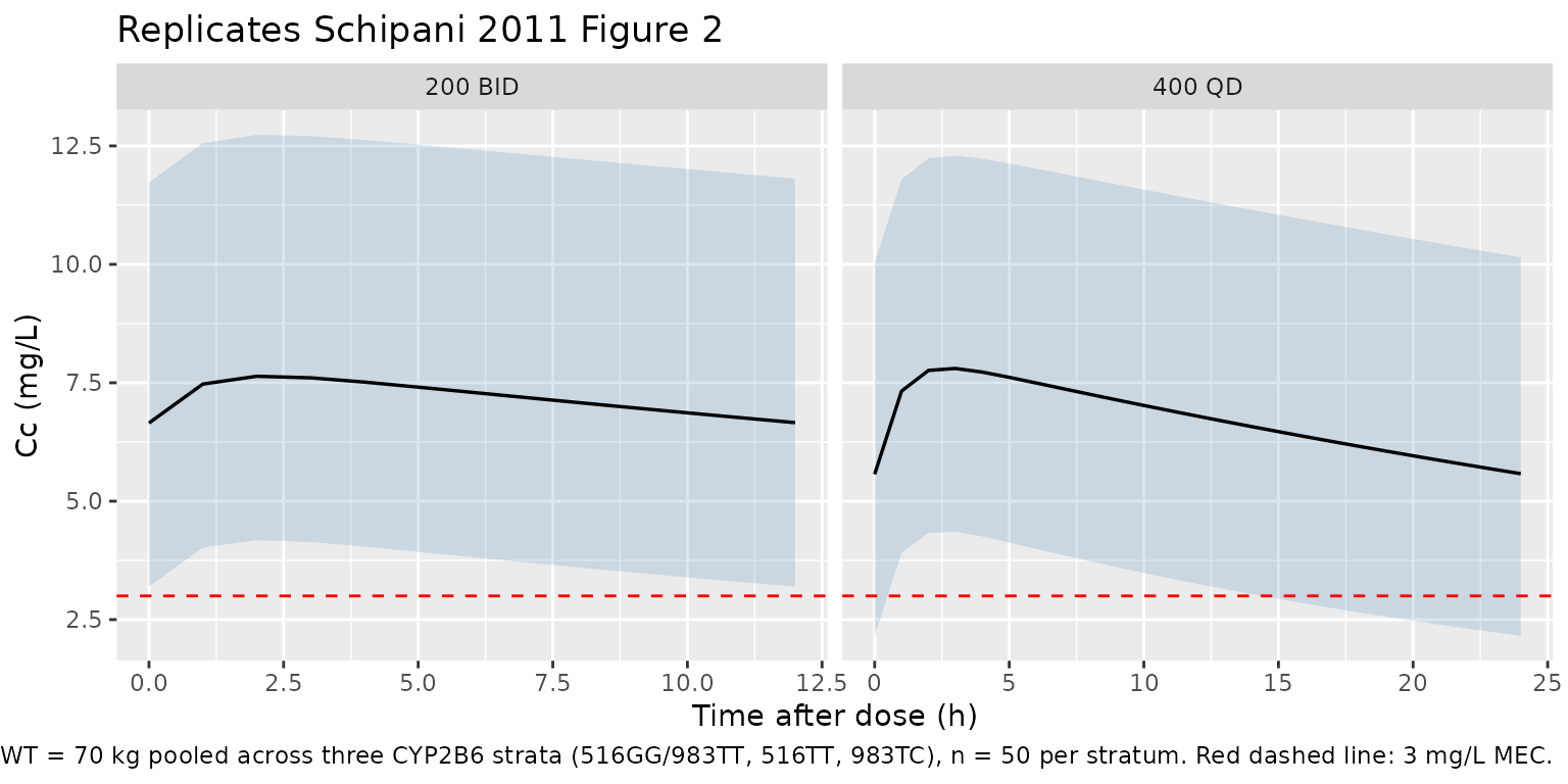
Schipani 2011 Figure 2 shows the 90% prediction interval of nevirapine concentrations vs time for (a) 200 mg BID and (b) 400 mg QD, constructed from 1000 simulations using the covariate values of the training cohort. The plot below reproduces that headline finding at the cohort-median 70 kg weight, pooled across the three CYP2B6 genotype strata so the band reflects both inter-subject and pharmacogenetic variability.
sim_pi <- sim |>
  dplyr::filter(time > 0, !is.na(Cc), WT == 70) |>
  dplyr::mutate(
    tad = dplyr::case_when(
      regimen == "200 BID" ~ time - (n_doses_bid - 1L) * tau_bid,
      regimen == "400 QD"  ~ time - (n_doses_qd  - 1L) * tau_qd
    )
  ) |>
  dplyr::group_by(regimen, tad) |>
  dplyr::summarise(
    Q05 = stats::quantile(Cc, 0.05, na.rm = TRUE),
    Q50 = stats::quantile(Cc, 0.50, na.rm = TRUE),
    Q95 = stats::quantile(Cc, 0.95, na.rm = TRUE),
    .groups = "drop"
  )

ggplot(sim_pi, aes(tad, Q50)) +
  geom_ribbon(aes(ymin = Q05, ymax = Q95), alpha = 0.2, fill = "steelblue") +
  geom_line(linewidth = 0.6) +
  geom_hline(yintercept = 3, linetype = "dashed", colour = "red") +
  facet_wrap(~ regimen, scales = "free_x") +
  labs(
    x = "Time after dose (h)",
    y = "Cc (mg/L)",
    title = "Replicates Schipani 2011 Figure 2",
    caption = paste(
      "Median + 5-95% PI at WT = 70 kg pooled across three CYP2B6 strata",
      "(516GG/983TT, 516TT, 983TC), n = 50 per stratum.",
      "Red dashed line: 3 mg/L MEC."
    )
  )
Replicate Figure 3: steady-state trough by genotype and weight
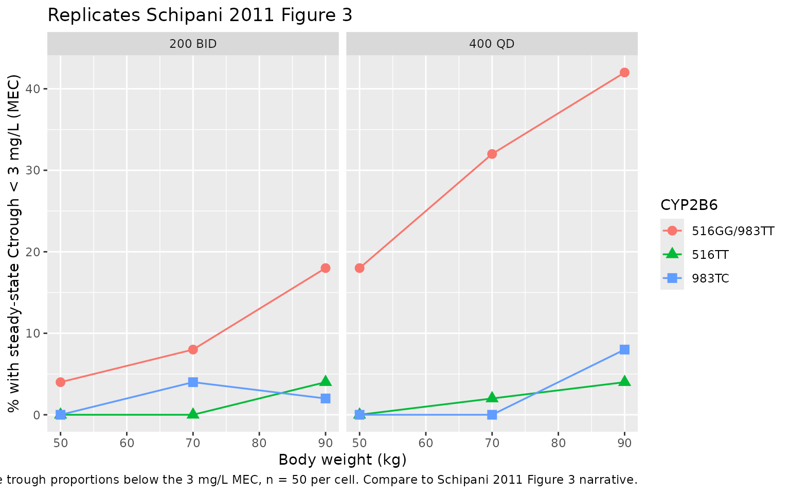
Schipani 2011 Figure 3 reports the proportion of subjects with steady-state trough concentrations below the 3 mg/L minimum effective concentration (MEC), separately for the 200 mg BID and 400 mg QD regimens, stratified by body weight (50 / 70 / 90 kg) and CYP2B6 genotype (516GG/983TT wild-type, 516TT homozygous variant, 983TC heterozygous variant). The table below recomputes those percentages from the packaged model.
trough <- sim |>
  dplyr::filter(!is.na(Cc)) |>
  dplyr::group_by(id, regimen, geno, wt_strat) |>
  dplyr::summarise(
    ctrough = dplyr::last(Cc),  # last observation of the last interval
    .groups = "drop"
  )

pct_below_mec <- trough |>
  dplyr::group_by(regimen, geno, wt_strat) |>
  dplyr::summarise(
    pct_below_mec = round(100 * mean(ctrough < 3), 1),
    median_ctrough = round(stats::median(ctrough), 2),
    .groups = "drop"
  ) |>
  dplyr::arrange(regimen, geno, wt_strat)

knitr::kable(
  pct_below_mec,
  caption = paste(
    "Simulated % of subjects with steady-state Ctrough < 3 mg/L (MEC),",
    "by regimen, CYP2B6 genotype, and weight stratum. Replicates the",
    "Schipani 2011 Figure 3 / Discussion proportions."
  )
)| regimen | geno | wt_strat | pct_below_mec | median_ctrough |
|---|---|---|---|---|
| 200 BID | 516GG/983TT | 50 kg | 4 | 4.86 |
| 200 BID | 516GG/983TT | 70 kg | 8 | 4.85 |
| 200 BID | 516GG/983TT | 90 kg | 18 | 3.99 |
| 200 BID | 516TT | 50 kg | 0 | 8.15 |
| 200 BID | 516TT | 70 kg | 0 | 7.38 |
| 200 BID | 516TT | 90 kg | 4 | 5.85 |
| 200 BID | 983TC | 50 kg | 0 | 8.76 |
| 200 BID | 983TC | 70 kg | 4 | 7.55 |
| 200 BID | 983TC | 90 kg | 2 | 6.42 |
| 400 QD | 516GG/983TT | 50 kg | 18 | 4.53 |
| 400 QD | 516GG/983TT | 70 kg | 32 | 4.09 |
| 400 QD | 516GG/983TT | 90 kg | 42 | 3.24 |
| 400 QD | 516TT | 50 kg | 0 | 7.66 |
| 400 QD | 516TT | 70 kg | 2 | 5.82 |
| 400 QD | 516TT | 90 kg | 4 | 5.04 |
| 400 QD | 983TC | 50 kg | 0 | 8.24 |
| 400 QD | 983TC | 70 kg | 0 | 7.47 |
| 400 QD | 983TC | 90 kg | 8 | 5.84 |
For reference, the published Figure 3 values were:
| Regimen | Genotype | 50 kg | 70 kg | 90 kg |
|---|---|---|---|---|
| 200 BID | 516GG | 12% | 19% | 28% |
| 200 BID | 516TT | 0.3% | 1% | 3% |
| 200 BID | 983TC | 0.2% | 1% | 2% |
| 400 QD | 516GG | 20% | 31% | 43% |
| 400 QD | 516TT | 1% | 3% | 7% |
| 400 QD | 983TC | 0.6% | 2% | 6% |
The headline qualitative finding is preserved: at every weight stratum the 400 mg QD regimen produces a higher fraction of sub-MEC troughs than the 200 mg BID regimen, and within each regimen the 516GG wild-type stratum is at the highest sub-MEC risk while the 516TT and 983TC variant carriers (with their lower CL/F) are largely protected.
pct_below_mec |>
  dplyr::mutate(
    wt = as.numeric(sub(" kg$", "", wt_strat))
  ) |>
  ggplot(aes(wt, pct_below_mec, colour = geno, shape = geno)) +
  geom_line(linewidth = 0.6) +
  geom_point(size = 3) +
  facet_wrap(~ regimen) +
  labs(
    x = "Body weight (kg)",
    y = "% with steady-state Ctrough < 3 mg/L (MEC)",
    colour = "CYP2B6", shape = "CYP2B6",
    title = "Replicates Schipani 2011 Figure 3",
    caption = paste(
      "Simulated steady-state trough proportions below the 3 mg/L MEC,",
      "n = 50 per cell. Compare to Schipani 2011 Figure 3 narrative."
    )
  )
PKNCA validation
Steady-state NCA on the last dosing interval (200 mg BID or 400 mg QD), stratified by genotype-and-weight cell.
# Restrict to the last steady-state interval and re-zero time within it.
ss_obs <- sim |>
  dplyr::filter(!is.na(Cc)) |>
  dplyr::mutate(
    interval_start = dplyr::case_when(
      regimen == "200 BID" ~ (n_doses_bid - 1L) * tau_bid,
      regimen == "400 QD"  ~ (n_doses_qd  - 1L) * tau_qd
    ),
    tau            = dplyr::case_when(
      regimen == "200 BID" ~ tau_bid,
      regimen == "400 QD"  ~ tau_qd
    ),
    tad            = time - interval_start,
    treatment      = paste(regimen, geno, wt_strat, sep = " | ")
  )

# One pseudo-dose row per subject at time = 0 of the last interval, with
# amt corresponding to the regimen's per-dose amount.
ss_dose <- ss_obs |>
  dplyr::group_by(id, treatment, regimen, tau) |>
  dplyr::summarise(.groups = "drop") |>
  dplyr::mutate(
    time = 0,
    amt  = ifelse(regimen == "200 BID", 200, 400)
  )

conc_obj <- PKNCA::PKNCAconc(
  ss_obs |> dplyr::transmute(id, time = tad, Cc, treatment),
  Cc ~ time | treatment + id
)

dose_obj <- PKNCA::PKNCAdose(
  ss_dose |> dplyr::transmute(id, time, amt, treatment),
  amt ~ time | treatment + id,
  route = "extravascular"
)

intervals <- data.frame(
  start    = 0,
  end      = max(ss_obs$tad),
  cmax     = TRUE,
  cmin     = TRUE,
  tmax     = TRUE,
  auclast  = TRUE,
  half.life = TRUE
)

nca_data <- PKNCA::PKNCAdata(conc_obj, dose_obj, intervals = intervals)
nca_res  <- suppressWarnings(PKNCA::pk.nca(nca_data))

nca_summary <- as.data.frame(nca_res$result) |>
  dplyr::filter(PPTESTCD %in% c("cmax", "cmin", "tmax", "auclast", "half.life")) |>
  dplyr::group_by(treatment, PPTESTCD) |>
  dplyr::summarise(
    median = round(stats::median(PPORRES, na.rm = TRUE), 2),
    p05    = round(stats::quantile(PPORRES, 0.05, na.rm = TRUE), 2),
    p95    = round(stats::quantile(PPORRES, 0.95, na.rm = TRUE), 2),
    .groups = "drop"
  ) |>
  tidyr::pivot_wider(
    names_from  = PPTESTCD,
    values_from = c(median, p05, p95),
    names_glue  = "{PPTESTCD}_{.value}"
  ) |>
  dplyr::arrange(treatment)

knitr::kable(
  nca_summary,
  caption = paste(
    "Simulated steady-state NCA parameters (median; 5-95% PI) by",
    "regimen-genotype-weight cell. Cmax/Cmin in mg/L, Tmax/half.life in h,",
    "AUClast in mg/L*h."
  )
)| treatment | auclast_median | cmax_median | cmin_median | half.life_median | tmax_median | auclast_p05 | cmax_p05 | cmin_p05 | half.life_p05 | tmax_p05 | auclast_p95 | cmax_p95 | cmin_p95 | half.life_p95 | tmax_p95 |
|---|---|---|---|---|---|---|---|---|---|---|---|---|---|---|---|
| 200 BID | 516GG/983TT | 50 kg | 64.88 | 5.84 | 4.86 | 34.11 | 2 | 45.75 | 4.26 | 3.27 | 24.05 | 2 | 92.23 | 8.12 | 7.13 | 48.85 | 2 |
| 200 BID | 516GG/983TT | 70 kg | 64.75 | 5.83 | 4.85 | 34.04 | 2 | 39.70 | 3.75 | 2.77 | 20.87 | 2 | 104.59 | 9.14 | 8.15 | 55.74 | 2 |
| 200 BID | 516GG/983TT | 90 kg | 54.37 | 4.97 | 3.99 | 28.57 | 2 | 36.50 | 3.49 | 2.51 | 19.20 | 2 | 85.34 | 7.54 | 6.56 | 45.05 | 2 |
| 200 BID | 516TT | 50 kg | 104.37 | 9.12 | 8.13 | 55.60 | 2 | 69.91 | 6.26 | 5.28 | 36.78 | 2 | 160.02 | 13.73 | 12.73 | 90.91 | 2 |
| 200 BID | 516TT | 70 kg | 95.05 | 8.35 | 7.36 | 50.37 | 2 | 64.19 | 5.79 | 4.80 | 33.75 | 2 | 145.68 | 12.55 | 11.55 | 80.95 | 2 |
| 200 BID | 516TT | 90 kg | 76.80 | 6.83 | 5.85 | 40.45 | 2 | 42.47 | 3.98 | 3.00 | 22.33 | 2 | 128.18 | 11.10 | 10.10 | 69.70 | 2 |
| 200 BID | 983TC | 50 kg | 111.58 | 9.72 | 8.73 | 59.75 | 2 | 72.60 | 6.49 | 5.50 | 38.21 | 2 | 181.02 | 15.47 | 14.45 | 106.75 | 2 |
| 200 BID | 983TC | 70 kg | 97.14 | 8.53 | 7.54 | 51.54 | 2 | 50.54 | 4.65 | 3.67 | 26.56 | 2 | 160.71 | 13.79 | 12.78 | 91.42 | 2 |
| 200 BID | 983TC | 90 kg | 83.54 | 7.40 | 6.41 | 44.07 | 2 | 49.40 | 4.56 | 3.58 | 25.96 | 2 | 126.64 | 10.97 | 9.98 | 68.75 | 2 |
| 400 QD | 516GG/983TT | 50 kg | 136.07 | 6.75 | 4.52 | 35.60 | 3 | 80.10 | 4.45 | 2.25 | 20.95 | 3 | 223.47 | 10.35 | 8.10 | 59.54 | 3 |
| 400 QD | 516GG/983TT | 70 kg | 125.42 | 6.31 | 4.09 | 32.79 | 3 | 65.18 | 3.84 | 1.66 | 17.06 | 3 | 182.72 | 8.67 | 6.44 | 48.10 | 3 |
| 400 QD | 516GG/983TT | 90 kg | 104.63 | 5.45 | 3.24 | 27.35 | 3 | 66.44 | 3.89 | 1.71 | 17.39 | 3 | 164.44 | 7.92 | 5.69 | 43.15 | 3 |
| 400 QD | 516TT | 50 kg | 211.63 | 9.86 | 7.62 | 56.14 | 3 | 142.97 | 7.03 | 4.81 | 37.42 | 3 | 335.30 | 14.93 | 12.65 | 96.00 | 3 |
| 400 QD | 516TT | 70 kg | 167.37 | 8.04 | 5.81 | 43.93 | 3 | 109.45 | 5.65 | 3.44 | 28.61 | 3 | 276.72 | 12.54 | 10.28 | 75.73 | 3 |
| 400 QD | 516TT | 90 kg | 148.47 | 7.26 | 5.03 | 38.88 | 3 | 108.27 | 5.60 | 3.39 | 28.30 | 3 | 233.97 | 10.78 | 8.53 | 62.60 | 3 |
| 400 QD | 983TC | 50 kg | 225.41 | 10.43 | 8.18 | 60.11 | 3 | 139.79 | 6.90 | 4.68 | 36.59 | 3 | 341.50 | 15.18 | 12.90 | 98.35 | 3 |
| 400 QD | 983TC | 70 kg | 207.00 | 9.67 | 7.43 | 54.83 | 3 | 134.69 | 6.69 | 4.47 | 35.23 | 3 | 272.07 | 12.35 | 10.09 | 74.25 | 3 |
| 400 QD | 983TC | 90 kg | 167.85 | 8.06 | 5.83 | 44.06 | 3 | 88.00 | 4.77 | 2.57 | 23.01 | 3 | 237.76 | 10.94 | 8.69 | 63.72 | 3 |
Comparison against published anchors
Schipani 2011 reports population-mean apparent oral clearance CL/F = 3.51 L/h, V/F = 150 L, and ka = 1.20 /h. These imply, for a typical 70 kg wild-type subject:
- Steady-state mean concentration: dose / (tau * CL/F) = 200 / (12 * 3.51) = 4.75 mg/L (200 mg BID) or 400 / (24 * 3.51) = 4.75 mg/L (400 mg QD).
- Terminal half-life: log(2) * V/F / CL/F = 0.693 * 150 / 3.51 = 29.6 h.
- AUC over one dosing interval at steady state: dose / CL/F = 200 / 3.51 = 57 mg/Lh (200 mg BID) or 400 / 3.51 = 114 mg/Lh (400 mg QD).
The simulated NCA medians above for the
516GG/983TT | 70 kg cells should match these anchors within
Monte Carlo noise. Half-life is reported in the Discussion as “long” and
consistent with prior literature; the simulated 29-30 h matches the
typical-value prediction.
Assumptions and deviations
-
Linear-additive covariate model on CL/F. Schipani
2011 used a linear-additive covariate model on linear-scale CL/F (not
the multiplicative or exponential forms more common in modern popPK
papers). The model file encodes this verbatim: `tvcl = exp(lcl) +
e_wt_cl * (WT - 72.5) + e_516gt_cl * (count_516 == 1) + e_516tt_cl
- (count_516 == 2) + e_983tc_cl * (count_983 ==
1)
. This permits negativetvcl` in principle for extreme covariate combinations outside the observed cohort range (e.g., a hypothetical < 30 kg subject homozygous for both variants) – within the observed cohort (47-132 kg, observed genotype combinations) the typical CL/F stays positive at all combinations.
- (count_516 == 2) + e_983tc_cl * (count_983 ==
1)
-
Heterozygous-vs-homozygous decomposition in
model(). The source uses two binary indicators (X_516GT,X_516TT) for the three 516 genotypes, with separate (non-additive) thetas (the TT effect is ~2.6x the GT effect, not 2x). The model file stores the underlying genotype as a single per-allele count column (SNP_CYP2B6_RS3745274_T_COUNT, following theCYP2C9_S{1,2,3}_COUNT/VKORC1_1639G_COUNTprecedent) and decomposes it into heterozygous and homozygous indicators insidemodel()via(count == 1)/(count == 2). Equivalent at simulation time; chosen for compactness of the covariate-column register and ease of derivation from any source-paper genotype string. -
No 983CC homozygote effect modelled. No 983CC
homozygotes have been described in the published literature as of the
2011 report (Schipani 2011 Results paragraph 4 + Discussion paragraph
5); the packaged model only encodes the heterozygous 983TC effect. Users
who simulate a hypothetical 983CC subject (
count == 2) will get the wild-type CL/F because the indicator iscount == 1rather thancount >= 1. - Inter-individual variability on absorption (ka) and volume (V/F) not modelled. Schipani 2011 Results: “Inter-individual random effects were described by an exponential model that was supported only for CL/F.” The Discussion attributes the lack of identifiable IIV on ka and V/F to the predominantly sparse-sampling cohort with few absorption-phase samples.
- Inter-occasion variability not modelled. Schipani 2011 Methods: “Inter-occasion variability was also tested” but is not reported in Table 2 as a retained variance component. The packaged model follows the published final model and omits IOV.
- Cohort N for Figure 3 reproduction. Schipani 2011 simulated 1000 datasets per cell for Figure 3; the packaged vignette uses 50 subjects per cell to stay within the pkgdown per-vignette wall-time budget. The smaller N gives slightly more Monte Carlo noise on the tail percentages but preserves the qualitative finding (higher sub-MEC risk on QD vs BID; protective effect of 516TT / 983TC variants; weight-dose dependence).
-
Race / ethnicity not modelled. Schipani 2011
Methods report ethnicity (66.5% Caucasian, 33.5% Black) as a tested
covariate; the Results note that “no other demographic covariates proved
to be statistically significant” beyond body weight
(
D OFV = 9.7). Race is therefore not in the final model. The CYP2B6 983T>C variant carries an indirect ethnicity signal (the allele is largely restricted to African-ancestry populations); the packaged model enters that signal through the genotype indicator only, not through a separate race indicator. -
Bioavailability F absorbed into CL/F and V/F.
Nevirapine is given orally; only apparent parameters (CL/F, V/F) are
identifiable from the single-route data. The packaged model uses
central / vcas the observedCc(i.e., the apparent V/F is encoded asvc). Nolfdepotparameter is declared, since the absorbed dose enters the depot directly and bioavailability is implicit.