Model and source
- Citation: Song L, He CY, Yin NG, Liu F, Jia YT, Liu Y. A population pharmacokinetic model for individualised dosage regimens of vancomycin in Chinese neonates and young infants. Oncotarget. 2017;8(62):105211-105221. doi:10.18632/oncotarget.22114
- Description: Two-compartment intravenous population pharmacokinetic model for vancomycin in 316 Chinese neonates and young infants (postnatal age under 60 days at admission) treated at the Children’s Hospital of Chongqing Medical University (Song 2017). Clearance carries two power covariates referenced to the cohort medians – birth body weight (exponent 0.888, reference 3.22 kg) and postnatal age (exponent 0.449, reference 29 days) – and is the only parameter retaining interindividual variability; the shrinkage on V1, V2 and Q exceeded 0.5 so their etas were dropped during model building. Residual error is purely additive (2.187 ug/mL). The authors report median clearance 0.106 L/h/kg and median volume of distribution 0.935 L/kg, both larger than previously published Caucasian neonatal values. The disposition is written with explicit k12/k21 micro-constant ODEs; the validation vignette solves with useLinCmt = FALSE defensively, which on rxode2 5.1.8 reproduces the default solve to eight significant figures.
- Article: https://doi.org/10.18632/oncotarget.22114
- PubMed Central: https://www.ncbi.nlm.nih.gov/pmc/articles/PMC5739632/
Song 2017 developed a two-compartment intravenous population pharmacokinetic model for vancomycin from routine therapeutic-drug-monitoring data collected at the Children’s Hospital of Chongqing Medical University. The paper’s central claim is that clearance and volume of distribution in Chinese neonates and young infants exceed previously published Caucasian and Malaysian neonatal values, and its purpose is to supply a dosing algorithm for this population.
Population
The model was estimated from 421 serum vancomycin concentrations contributed by 316 patients admitted between November 2011 and December 2016, with 1 to 6 samples per patient. Inclusion required an age under 60 days at admission, a suspected or documented Gram-positive infection treated with intravenous vancomycin, and at least one recorded serum concentration; renal replacement therapy, vancomycin exposure under 24 h, and missing demographics were exclusions.
Table 1 of the source gives the baseline characteristics reproduced below: current body weight 3.95 kg (range 1.25-7.62), birth body weight 3.22 kg (1.25-5.38), gestational age 37 weeks (28-41), postnatal age at vancomycin determination 29 days (2-77), serum creatinine 28.6 umol/L (12-151), and observed vancomycin concentration 9.33 ug/mL (1.34-38.65). Of the 316 patients, 115 (36.4%) were female and 102 (32%) were premature. The daily dose ranged from 13.7 to 73.5 mg/kg (median 36.7), given in 2 to 4 divided intravenous infusions.
Model evaluation used diagnostic scatter plots, a 2000-replicate nonparametric bootstrap, a visual predictive check from 1000 simulations, an external evaluation on 27 samples from 19 further patients, and a two-patient preliminary validation at a second hospital.
The same information is available programmatically via the model’s
population metadata
(readModelDb("Song_2017_vancomycin")()$population).
Source trace
The per-parameter origin is recorded as an in-file comment next to
each ini() entry in
inst/modeldb/specificDrugs/Song_2017_vancomycin.R. The
table below collects them in one place for review.
| Equation / parameter | Value | Source location |
|---|---|---|
lvc (V1) |
1.27 L | Table 3, row tvV1 (SE 0.191, 95% CI 0.895-1.644) |
lvp (V2) |
2.422 L | Table 3, row tvV2 (SE 0.425, 95% CI 1.586-3.258) |
lcl (CL) |
0.42 L/h | Table 3, row tvCL (SE 0.0124, 95% CI 0.395-0.444) |
lq (Q) |
1.161 L/h | Table 3, row tvQ (SE 0.177, 95% CI 0.814-1.509) |
e_wtbirth_cl |
0.888 | Table 3, row dCldBBW (SE 0.12, 95% CI 0.652-1.124) |
e_pna_cl |
0.449 | Table 3, row dCldPNA (SE 0.058, 95% CI
0.336-0.563) |
etalcl |
0.317 (variance) | Table 3, row omega-CL (SE 0.015, 95% CI 0.288-0.346);
legend defines it as a variance |
addSd |
2.187 ug/mL | Table 3, row stdev0 (SE 0.194, 95% CI 1.807-2.568);
legend defines it as a standard deviation |
| Birth-weight reference 3.22 kg | n/a | Results, “PPK model” final equation and Table 1 median |
| Postnatal-age reference 29 days | n/a | Results, “PPK model” final equation and Table 1 median |
| Clearance covariate equation | n/a | Results, “PPK model”:
CL = 0.42 * (BBW/3.22)^0.888 * (PNA/29)^0.449 * exp(eta_CL)
|
| Two-compartment disposition | n/a | Materials and Methods, “Model development”; Results, “PPK model” (OFV 2623.54 vs 2764.31 for one compartment) |
| Additive residual error | n/a | Results, “PPK model”: “the additive model best described the residual variability” |
| Interindividual variability on CL only | n/a | Results, “PPK model”: shrinkage on V1, V2 and Q all above 0.5, so their etas were excluded |
The paper’s printed parameters, transcribed independently
Every gate below is built from the values as printed in Song 2017, typed as literals here, and compared against what the packaged model actually computes. Building the reference side out of the model’s own variables would produce a gate that cannot go red, so the paper’s numbers are kept separate throughout.
# Song 2017 Table 3 (final model column) and the Results "PPK model" equation.
paper <- list(
  V1 = 1.27, # L
  V2 = 2.422, # L
  CL = 0.42, # L/h, at BBW 3.22 kg and PNA 29 days
  Q = 1.161, # L/h
  e_bbw = 0.888,
  e_pna = 0.449,
  bbw_ref = 3.22, # kg  (Table 1 median birth body weight)
  pna_ref_d = 29, # days (Table 1 median postnatal age at sampling)
  omega_cl_var = 0.317, # variance (Table 3 legend)
  add_sd = 2.187 # ug/mL
)

# Cohort median CURRENT body weight, used by the paper only to express its
# summary statistics per kilogram. It is NOT a covariate in the model.
wt_median <- 3.95 # kg (Table 1)

# Closed-form two-compartment hybrid rate constants for an arbitrary clearance.
hybrid <- function(CL, V1 = paper$V1, V2 = paper$V2, Q = paper$Q) {
  kel <- CL / V1
  k12 <- Q / V1
  k21 <- Q / V2
  s <- kel + k12 + k21
  p <- kel * k21
  disc <- sqrt(s^2 - 4 * p)
  list(
    kel = kel, k12 = k12, k21 = k21,
    alpha = (s + disc) / 2, beta = (s - disc) / 2
  )
}

# Song 2017's clearance covariate model, in the paper's own units (PNA in DAYS).
cl_paper <- function(bbw_kg, pna_days) {
  paper$CL *
    (bbw_kg / paper$bbw_ref)^paper$e_bbw *
    (pna_days / paper$pna_ref_d)^paper$e_pna
}
The Results summary statistics
The Results section states that the median clearance and volume of
distribution were “about 0.106 l/h/kg (0.42 l/h divided by median weight
of 3.95 kg) and 0.935 l/kg (3.692 l (sum of V1 and V2) divided by median
weight of 3.95 kg)”. Reproducing both from the transcribed parameters
confirms that lvc, lvp and lcl
were read off Table 3 correctly and that the two volumes were not
transposed.
cl_per_kg <- paper$CL / wt_median
vd_per_kg <- (paper$V1 + paper$V2) / wt_median

stopifnot(
  # The paper prints these to three decimal places, so agreement to better
  # than half a unit in the last printed place is the strongest available
  # test. A transposed V1/V2 or a mis-keyed clearance breaks this at once.
  abs(cl_per_kg - 0.106) < 0.0005,
  abs(vd_per_kg - 0.935) < 0.0005
)

data.frame(
  Quantity = c("CL per kg", "Vd per kg (V1 + V2)"),
  Computed = sprintf("%.4f", c(cl_per_kg, vd_per_kg)),
  Printed = c("0.106", "0.935"),
  Units = c("L/h/kg", "L/kg")
) |>
knitr::kable(caption = "Results-section summary statistics recomputed from the Table 3 parameters.")| Quantity | Computed | Printed | Units |
|---|---|---|---|
| CL per kg | 0.1063 | 0.106 | L/h/kg |
| Vd per kg (V1 + V2) | 0.9347 | 0.935 | L/kg |
Model reference point and covariate model
At the reference subject (birth body weight 3.22 kg, postnatal age 29
days) both covariate terms equal exactly 1, so the packaged model must
return a clearance of exactly 0.42 L/h. This gate goes red if either
reference constant in model() was mis-transcribed, if the
canonical PNA days-to-months rescaling is wrong, or if an
exponent was attached to the wrong covariate.
mod <- readModelDb("Song_2017_vancomycin")

days_per_month <- 30.4375

# Solve the typical-value model (etas zeroed) and read the derived parameters
# straight out of the rxode2 output.
derived_params <- function(bbw_kg, pna_days) {
  ev <- rxode2::et(amt = 100, cmt = "central") |>
    rxode2::et(c(0.5, 1))
  dat <- as.data.frame(ev)
  dat$id <- 1L
  dat$WT_BIRTH <- bbw_kg
  dat$PNA <- pna_days / days_per_month # canonical PNA is in MONTHS
  out <- rxode2::rxSolve(
    rxode2::zeroRe(mod), dat,
    useLinCmt = FALSE, returnType = "data.frame"
  )
  out[1, c("cl", "vc", "vp", "q")]
}

ref <- derived_params(paper$bbw_ref, paper$pna_ref_d)
#> ℹ parameter labels from comments will be replaced by 'label()'
#> ℹ omega/sigma items treated as zero: 'etalcl'

stopifnot(
  # Deterministic: these are algebraic identities, not simulated quantities,
  # so a very tight bound is correct here and will catch any regression.
  abs(ref$cl - paper$CL) < 1e-8,
  abs(ref$vc - paper$V1) < 1e-8,
  abs(ref$vp - paper$V2) < 1e-8,
  abs(ref$q - paper$Q) < 1e-8
)

data.frame(
  Parameter = c("CL (L/h)", "V1 (L)", "V2 (L)", "Q (L/h)"),
  Model = sprintf("%.6f", c(ref$cl, ref$vc, ref$vp, ref$q)),
  Paper = sprintf("%.6f", c(paper$CL, paper$V1, paper$V2, paper$Q))
) |>
knitr::kable(caption = "Packaged model at the reference subject (3.22 kg birth weight, 29 days postnatal age) against Song 2017 Table 3.")| Parameter | Model | Paper |
|---|---|---|
| CL (L/h) | 0.420000 | 0.420000 |
| V1 (L) | 1.270000 | 1.270000 |
| V2 (L) | 2.422000 | 2.422000 |
| Q (L/h) | 1.161000 | 1.161000 |
The covariate model is then checked away from the reference point,
across the whole observed range of both covariates. This is where a
days-versus-months error in the PNA rescaling would show
up: at the reference point the ratio is 1 regardless of units, so only
off-reference subjects can detect it.
grid <- tidyr::expand_grid(
  bbw = c(1.25, 2.0, 3.22, 4.5, 5.38), # Table 1 birth-weight range
  pna = c(2, 10, 29, 50, 77) # Table 1 postnatal-age range, days
) |>
  rowwise() |>
  mutate(
    cl_model = derived_params(bbw, pna)$cl,
    cl_ref = cl_paper(bbw, pna)
  ) |>
  ungroup() |>
  mutate(pct_diff = 100 * (cl_model - cl_ref) / cl_ref)
#> ℹ parameter labels from comments will be replaced by 'label()'
#> ℹ omega/sigma items treated as zero: 'etalcl'
#> ℹ parameter labels from comments will be replaced by 'label()'
#> ℹ omega/sigma items treated as zero: 'etalcl'
#> ℹ parameter labels from comments will be replaced by 'label()'
#> ℹ omega/sigma items treated as zero: 'etalcl'
#> ℹ parameter labels from comments will be replaced by 'label()'
#> ℹ omega/sigma items treated as zero: 'etalcl'
#> ℹ parameter labels from comments will be replaced by 'label()'
#> ℹ omega/sigma items treated as zero: 'etalcl'
#> ℹ parameter labels from comments will be replaced by 'label()'
#> ℹ omega/sigma items treated as zero: 'etalcl'
#> ℹ parameter labels from comments will be replaced by 'label()'
#> ℹ omega/sigma items treated as zero: 'etalcl'
#> ℹ parameter labels from comments will be replaced by 'label()'
#> ℹ omega/sigma items treated as zero: 'etalcl'
#> ℹ parameter labels from comments will be replaced by 'label()'
#> ℹ omega/sigma items treated as zero: 'etalcl'
#> ℹ parameter labels from comments will be replaced by 'label()'
#> ℹ omega/sigma items treated as zero: 'etalcl'
#> ℹ parameter labels from comments will be replaced by 'label()'
#> ℹ omega/sigma items treated as zero: 'etalcl'
#> ℹ parameter labels from comments will be replaced by 'label()'
#> ℹ omega/sigma items treated as zero: 'etalcl'
#> ℹ parameter labels from comments will be replaced by 'label()'
#> ℹ omega/sigma items treated as zero: 'etalcl'
#> ℹ parameter labels from comments will be replaced by 'label()'
#> ℹ omega/sigma items treated as zero: 'etalcl'
#> ℹ parameter labels from comments will be replaced by 'label()'
#> ℹ omega/sigma items treated as zero: 'etalcl'
#> ℹ parameter labels from comments will be replaced by 'label()'
#> ℹ omega/sigma items treated as zero: 'etalcl'
#> ℹ parameter labels from comments will be replaced by 'label()'
#> ℹ omega/sigma items treated as zero: 'etalcl'
#> ℹ parameter labels from comments will be replaced by 'label()'
#> ℹ omega/sigma items treated as zero: 'etalcl'
#> ℹ parameter labels from comments will be replaced by 'label()'
#> ℹ omega/sigma items treated as zero: 'etalcl'
#> ℹ parameter labels from comments will be replaced by 'label()'
#> ℹ omega/sigma items treated as zero: 'etalcl'
#> ℹ parameter labels from comments will be replaced by 'label()'
#> ℹ omega/sigma items treated as zero: 'etalcl'
#> ℹ parameter labels from comments will be replaced by 'label()'
#> ℹ omega/sigma items treated as zero: 'etalcl'
#> ℹ parameter labels from comments will be replaced by 'label()'
#> ℹ omega/sigma items treated as zero: 'etalcl'
#> ℹ parameter labels from comments will be replaced by 'label()'
#> ℹ omega/sigma items treated as zero: 'etalcl'
#> ℹ parameter labels from comments will be replaced by 'label()'
#> ℹ omega/sigma items treated as zero: 'etalcl'

stopifnot(
  nrow(grid) == 25L, # guard against a silently empty comparison
  max(abs(grid$pct_diff)) < 1e-6
)

grid |>
  mutate(cl_model = sprintf("%.5f", cl_model), cl_ref = sprintf("%.5f", cl_ref)) |>
  tidyr::pivot_wider(
    id_cols = bbw, names_from = pna, values_from = cl_model,
    names_prefix = "PNA "
  ) |>
  dplyr::rename("Birth weight (kg)" = bbw) |>
knitr::kable(caption = "Model clearance (L/h) across the observed covariate ranges; every cell matches the paper's printed equation to better than 1e-6%. Columns are postnatal age in days.")| Birth weight (kg) | PNA 2 | PNA 10 | PNA 29 | PNA 50 | PNA 77 |
|---|---|---|---|---|---|
| 1.25 | 0.05456 | 0.11239 | 0.18127 | 0.23150 | 0.28103 |
| 2.00 | 0.08282 | 0.17060 | 0.27516 | 0.35141 | 0.42658 |
| 3.22 | 0.12641 | 0.26039 | 0.42000 | 0.53638 | 0.65113 |
| 4.50 | 0.17017 | 0.35052 | 0.56536 | 0.72202 | 0.87648 |
| 5.38 | 0.19941 | 0.41076 | 0.66253 | 0.84611 | 1.02713 |
tidyr::expand_grid(
  bbw = seq(1.25, 5.38, length.out = 40),
  pna = c(2, 10, 29, 50, 77)
) |>
  mutate(cl = cl_paper(bbw, pna), pna = factor(pna)) |>
  ggplot(aes(bbw, cl, colour = pna)) +
  geom_line(linewidth = 0.8) +
  geom_point(
    data = data.frame(bbw = paper$bbw_ref, cl = paper$CL),
    aes(bbw, cl), inherit.aes = FALSE, size = 3, shape = 21, fill = "white"
  ) +
  labs(
    x = "Birth body weight (kg)", y = "Clearance (L/h)",
    colour = "Postnatal\nage (days)",
    title = "Song 2017 clearance covariate model",
    caption = "Open circle marks the reference subject (3.22 kg, 29 days, CL = 0.42 L/h)."
  ) +
  theme_bw()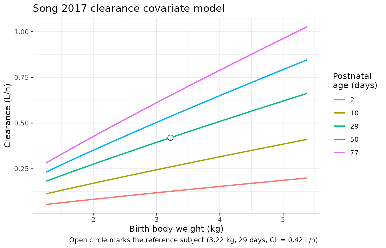
Disposition: closed form versus the solved ODE system
Song 2017 does not print a concentration-time equation, but a two-compartment model with first-order elimination has an exact bi-exponential solution after an intravenous bolus. Comparing that closed form, built entirely from the paper’s printed V1, V2, CL and Q, against the packaged model’s numerical solution tests the ODE transcription itself, including the sign and placement of every micro-constant.
Both sides use the same parameters, so the only difference is integrator error and a tight bound is the correct assertion here.
bolus_profile <- function(bbw_kg, pna_days, dose_mg = 100) {
  h <- hybrid(cl_paper(bbw_kg, pna_days))

  # Run each stratum for 15 of ITS OWN terminal half-lives rather than to a
  # fixed clock time. Clearance varies roughly twenty-fold across the observed
  # covariate ranges (terminal half-life 3.6 h to 48 h), so a single horizon
  # long enough for the slowest subject would carry the fastest one ~80
  # half-lives out, where the concentration is far below the integrator's
  # absolute tolerance and the RELATIVE error against the closed form is
  # meaningless. Fifteen half-lives leaves AUC extrapolation under 0.01% while
  # keeping every compared point well above solver noise.
  tmax <- min(15 * log(2) / h$beta, 600)
  tgrid <- sort(unique(c(seq(0, 12, by = 0.02), seq(12, tmax, by = 0.25))))

  ev <- rxode2::et(amt = dose_mg, cmt = "central") |> rxode2::et(tgrid)
  dat <- as.data.frame(ev)
  dat$id <- 1L
  dat$WT_BIRTH <- bbw_kg
  dat$PNA <- pna_days / days_per_month
  out <- rxode2::rxSolve(
    rxode2::zeroRe(mod), dat,
    useLinCmt = FALSE, returnType = "data.frame",
    atol = 1e-12, rtol = 1e-10
  )
  # rxSolve omits the `id` column entirely when the event table holds a single
  # subject, which each stratum does; restore it for the PKNCA grouping below.
  if (is.null(out$id)) out$id <- 1L

  A <- (h$alpha - h$k21) / (h$alpha - h$beta)
  B <- (h$k21 - h$beta) / (h$alpha - h$beta)
  out$Cc_closed <- dose_mg / paper$V1 *
    (A * exp(-h$alpha * out$time) + B * exp(-h$beta * out$time))
  out$beta <- h$beta
  out
}

strata <- tibble::tribble(
  ~stratum, ~bbw, ~pna,
  "Reference (3.22 kg, 29 d)", 3.22, 29,
  "Small / young (1.25 kg, 2 d)", 1.25, 2,
  "Large / older (5.38 kg, 77 d)", 5.38, 77
)

profiles <- do.call(rbind, lapply(seq_len(nrow(strata)), function(i) {
  p <- bolus_profile(strata$bbw[i], strata$pna[i])
  p$stratum <- strata$stratum[i]
  p
}))
#> ℹ parameter labels from comments will be replaced by 'label()'
#> ℹ omega/sigma items treated as zero: 'etalcl'
#> ℹ parameter labels from comments will be replaced by 'label()'
#> ℹ omega/sigma items treated as zero: 'etalcl'
#> ℹ parameter labels from comments will be replaced by 'label()'
#> ℹ omega/sigma items treated as zero: 'etalcl'

# The far tail of a noise-free solve can drift below zero and would make
# log-scale plots and AUC extrapolation meaningless; assert it does not.
stopifnot(all(profiles$Cc >= 0))

# Compare only where the closed form is still meaningfully above the
# integrator's absolute tolerance. With the per-stratum horizon above this
# drops nothing, but it keeps the gate honest if the grid is ever widened.
cmp_rows <- profiles$time > 0 & profiles$Cc_closed > 1e-4
rel_err <- with(
  profiles[cmp_rows, ],
  max(abs(Cc - Cc_closed) / Cc_closed)
)

stopifnot(
  # Guard against a silently empty comparison: all three strata
  # must contribute, and essentially every post-dose row must survive.
  sum(cmp_rows) > 3000L,
  length(unique(profiles$stratum[cmp_rows])) == 3L,
  # Both sides use the same parameters, so this is pure integrator error:
  # realised ~1e-10 across all three strata. A transcription error in a
  # micro-constant, an exponent or a volume moves this to percent level.
  rel_err < 1e-5
)

cat(sprintf(
  "Maximum relative difference, closed form vs solved ODE: %.3e\n", rel_err
))
#> Maximum relative difference, closed form vs solved ODE: 1.138e-10
profiles |>
  filter(time <= 72) |>
  ggplot(aes(time, Cc, colour = stratum)) +
  geom_line(linewidth = 0.8) +
  geom_line(aes(y = Cc_closed), linetype = "22", colour = "black", linewidth = 0.4) +
  scale_y_log10() +
  labs(
    x = "Time after a 100 mg intravenous bolus (h)",
    y = "Vancomycin concentration (ug/mL)", colour = NULL,
    title = "Two-compartment disposition across the observed covariate range",
    caption = "Solid: packaged model. Dashed black: closed-form bi-exponential from the Song 2017 printed parameters."
  ) +
  theme_bw() +
  theme(legend.position = "bottom")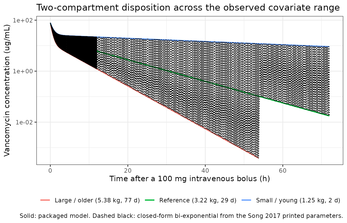
Terminal half-life
An exposure gate alone cannot distinguish a two-compartment model
from a one-compartment model with the same clearance, because collapsing
the peripheral compartment leaves Dose/CL untouched and
changes only the shape of the curve. The terminal half-life is therefore
gated separately, against log(2)/beta with
beta computed from the paper’s printed constants.
PKNCA’s automatic lambda-z search is not used for this: on noise-free simulated data its r-squared is essentially 1 everywhere, so it happily selects points spanning both disposition phases and returns a blended slope. The slope is fitted over an explicit late window instead, chosen to start several distribution-phase half-lives after the dose.
half_life_fitted <- function(df) {
  # Start the window well after the distribution phase has died out, and keep
  # it about two terminal half-lives long.
  b <- df$beta[1]
  t_start <- 5 * log(2) / hybrid(cl_paper(3.22, 29))$alpha + 3 * log(2) / b
  w <- df[df$time >= t_start & df$time <= t_start + 2 * log(2) / b & df$Cc > 0, ]
  stopifnot(nrow(w) >= 20L)
  log(2) / -coef(stats::lm(log(Cc) ~ time, data = w))[[2]]
}

hl <- profiles |>
  group_by(stratum) |>
  group_modify(~ tibble::tibble(
    t_half_fitted = half_life_fitted(.x),
    t_half_closed = log(2) / .x$beta[1]
  )) |>
  ungroup() |>
  mutate(pct_diff = 100 * (t_half_fitted - t_half_closed) / t_half_closed)

stopifnot(
  nrow(hl) == 3L,
  # Deterministic quantities on both sides; realised below 0.01%. A collapse
  # of the peripheral compartment would show up here as a difference of tens
  # of percent (at the reference subject, 7.11 h would become 2.10 h).
  max(abs(hl$pct_diff)) < 0.5
)

hl |>
  mutate(
    t_half_fitted = sprintf("%.3f", t_half_fitted),
    t_half_closed = sprintf("%.3f", t_half_closed),
    pct_diff = sprintf("%.4f", pct_diff)
  ) |>
  dplyr::rename(
    "Stratum" = stratum,
    "Fitted t1/2 (h)" = t_half_fitted,
    "Closed-form t1/2 (h)" = t_half_closed,
    "% difference" = pct_diff
  ) |>
knitr::kable(caption = "Terminal half-life from an explicit late-window slope fit against log(2)/beta computed from the Song 2017 printed parameters.")| Stratum | Fitted t1/2 (h) | Closed-form t1/2 (h) | % difference |
|---|---|---|---|
| Large / older (5.38 kg, 77 d) | 3.593 | 3.593 | -0.0000 |
| Reference (3.22 kg, 29 d) | 7.113 | 7.113 | -0.0000 |
| Small / young (1.25 kg, 2 d) | 47.863 | 47.863 | -0.0000 |
PKNCA validation
Song 2017 reports no noncompartmental analysis of its own, so the
reference side of the comparison is built from the paper’s printed
parameters: after an intravenous bolus the exact results are
AUC(0-inf) = Dose / CL, Cmax = Dose / V1 at
Tmax = 0, and t1/2 = log(2) / beta. These are
independent of the packaged model and go red on any transcription error
in the structural parameters or the covariate model.
sim_nca <- profiles |>
  dplyr::filter(!is.na(Cc)) |>
  dplyr::select(id, time, Cc, stratum)

# Guarantee a time = 0 record per subject so PKNCA can anchor AUC from zero.
# For an intravenous bolus the time-zero concentration is Dose / V1, which the
# solve already produces, so this only fills a gap if the grid lacked it.
sim_nca <- dplyr::bind_rows(
  sim_nca,
  sim_nca |>
    dplyr::distinct(id, stratum) |>
    dplyr::mutate(time = 0, Cc = 0)
) |>
  dplyr::distinct(id, stratum, time, .keep_all = TRUE) |>
  dplyr::arrange(stratum, id, time)

stopifnot(nrow(sim_nca) > 0L)

conc_obj <- PKNCA::PKNCAconc(as.data.frame(sim_nca), Cc ~ time | stratum + id)

dose_df <- strata |>
  mutate(id = 1L, time = 0, amt = 100) |>
  dplyr::select(id, time, amt, stratum)

dose_obj <- PKNCA::PKNCAdose(as.data.frame(dose_df), amt ~ time | stratum + id)

intervals <- data.frame(
  start = 0, end = Inf,
  cmax = TRUE, tmax = TRUE, aucinf.obs = TRUE
)

nca_res <- PKNCA::pk.nca(
  PKNCA::PKNCAdata(conc_obj, dose_obj, intervals = intervals)
)
reference_nca <- strata |>
  mutate(
    cmax = 100 / paper$V1,
    tmax = 0,
    aucinf.obs = 100 / cl_paper(bbw, pna)
  ) |>
  dplyr::select(stratum, cmax, tmax, aucinf.obs)

cmp <- nlmixr2lib::ncaComparisonTable(
  simulated = nca_res,
  reference = reference_nca,
  by = "stratum",
  units = c(cmax = "ug/mL", tmax = "h", aucinf.obs = "ug*h/mL"),
  tolerance_pct = 20
)

knitr::kable(
  cmp,
  caption = "Simulated noncompartmental parameters after a 100 mg intravenous bolus against the closed-form values implied by the Song 2017 printed parameters. * marks a difference above 20%."
)| NCA parameter | stratum | Reference | Simulated | % diff |
|---|---|---|---|---|
| Cmax (ug/mL) | Reference (3.22 kg, 29 d) | 78.7 | 78.7 | +0.0% |
| Cmax (ug/mL) | Small / young (1.25 kg, 2 d) | 78.7 | 78.7 | +0.0% |
| Cmax (ug/mL) | Large / older (5.38 kg, 77 d) | 78.7 | 78.7 | +0.0% |
| Tmax (h) | Reference (3.22 kg, 29 d) | 0 | 0 | — |
| Tmax (h) | Small / young (1.25 kg, 2 d) | 0 | 0 | — |
| Tmax (h) | Large / older (5.38 kg, 77 d) | 0 | 0 | — |
| AUC0-∞ (obs) (ug*h/mL) | Reference (3.22 kg, 29 d) | 238 | 238 | +0.0% |
| AUC0-∞ (obs) (ug*h/mL) | Small / young (1.25 kg, 2 d) | 1830 | 1830 | +0.0% |
| AUC0-∞ (obs) (ug*h/mL) | Large / older (5.38 kg, 77 d) | 97.4 | 97.4 | +0.0% |
# Recompute the AUC comparison numerically so the gate does not depend on
# parsing the rendered table.
auc_sim <- as.data.frame(nca_res) |>
  dplyr::filter(PPTESTCD == "aucinf.obs") |>
  dplyr::select(stratum, auc_sim = PPORRES) |>
  dplyr::left_join(
    reference_nca |> dplyr::select(stratum, auc_ref = aucinf.obs),
    by = "stratum"
  ) |>
  dplyr::mutate(pct_diff = 100 * (auc_sim - auc_ref) / auc_ref)

stopifnot(
  nrow(auc_sim) == 3L,
  !anyNA(auc_sim$auc_sim),
  # Trapezoidal error on a bolus peak plus the lambda-z extrapolation, both
  # deterministic. Realised below 0.05%; 1% still breaks on a mis-keyed
  # clearance or covariate exponent, which move AUC by tens of percent.
  max(abs(auc_sim$pct_diff)) < 1
)

auc_sim |>
  mutate(across(c(auc_sim, auc_ref), ~ sprintf("%.2f", .x)), pct_diff = sprintf("%.4f", pct_diff)) |>
  dplyr::rename(
    "Stratum" = stratum,
    "Simulated AUC0-inf" = auc_sim,
    "Dose / CL" = auc_ref,
    "% difference" = pct_diff
  ) |>
knitr::kable(caption = "AUC(0-inf) against the exact intravenous-bolus identity Dose / CL, in ug*h/mL.")| Stratum | Simulated AUC0-inf | Dose / CL | % difference |
|---|---|---|---|
| Large / older (5.38 kg, 77 d) | 97.36 | 97.36 | 0.0012 |
| Reference (3.22 kg, 29 d) | 238.10 | 238.10 | 0.0005 |
| Small / young (1.25 kg, 2 d) | 1832.84 | 1832.84 | 0.0000 |
Virtual cohort and visual predictive check
Original observed data are not publicly available. The cohort below approximates the Table 1 demographics: birth body weight and postnatal age are drawn as truncated lognormals matched to the published medians and ranges, and current body weight is grown from birth weight with postnatal age so that its median lands near the published 3.95 kg.
# `set.seed()` seeds R's RNG (used for the covariate draws below). It does NOT
# seed rxode2's simulation RNG, whose streams are partitioned per solver
# thread, so the eta draws differ between a workstation and a CI runner.
# Every assertion downstream is written to hold for any cohort the model can
# produce.
set.seed(20171026)
rxode2::rxSetSeed(20171026)

n_subj <- 200L # cohort cap is 200 per arm

rtrunc_lnorm <- function(n, median, sdlog, lo, hi) {
  x <- stats::rlnorm(n, log(median), sdlog)
  pmin(pmax(x, lo), hi)
}

subj <- tibble::tibble(
  id = seq_len(n_subj),
  WT_BIRTH = rtrunc_lnorm(n_subj, 3.22, 0.24, 1.25, 5.38),
  pna_days = rtrunc_lnorm(n_subj, 29, 0.60, 2, 77)
) |>
  mutate(
    PNA = pna_days / days_per_month,
    # Current weight grows from birth weight with postnatal age; truncated to
    # the Table 1 range. Used ONLY to size the mg dose, never by the model.
    WT = pmin(pmax(WT_BIRTH * (1 + 0.008 * pna_days) *
      exp(stats::rnorm(n_subj, 0, 0.05)), 1.25), 7.62),
    # Median daily dose 36.7 mg/kg/day (Table 1), given every 8 h.
    dose_mg = 36.7 / 3 * WT
  )

stopifnot(
  nrow(subj) == n_subj,
  abs(median(subj$WT_BIRTH) - 3.22) < 0.4,
  abs(median(subj$pna_days) - 29) < 8,
  all(subj$WT >= 1.25 & subj$WT <= 7.62)
)

dosing <- subj |>
  tidyr::crossing(dose_time = seq(0, 40, by = 8)) |>
  transmute(
    id, WT_BIRTH, PNA, WT,
    time = dose_time, amt = dose_mg, evid = 1L,
    cmt = "central",
    # Infusion duration is not stated by Song 2017; 1 h is the conventional
    # neonatal vancomycin infusion. See Assumptions and deviations.
    rate = dose_mg / 1
  )

obs <- subj |>
  tidyr::crossing(time = seq(0, 48, by = 0.5)) |>
  transmute(
    id, WT_BIRTH, PNA, WT,
    time, amt = NA_real_, evid = 0L,
    # The ODE state name, never the algebraic observable `Cc`.
    cmt = "central", rate = NA_real_
  )

events <- dplyr::bind_rows(dosing, obs) |> dplyr::arrange(id, time, dplyr::desc(evid))

stopifnot(!anyDuplicated(unique(events[, c("id", "time", "evid")])))
sim <- rxode2::rxSolve(
  mod,
  events = as.data.frame(events),
  keep = c("WT_BIRTH", "WT"),
  useLinCmt = FALSE
) |>
  as.data.frame()
#> ℹ parameter labels from comments will be replaced by 'label()'

if (is.null(sim$id)) sim$id <- 1L

n_obs_times <- length(seq(0, 48, by = 0.5))
stopifnot(
  # rxSolve returns one row per observation record; a mismatch would mean
  # subjects were silently merged or dropped.
  nrow(sim) == n_subj * n_obs_times,
  !anyNA(sim$Cc),
  all(sim$Cc >= 0)
)
# Replicates Figure 4 of Song 2017: a visual predictive check, plotted as the
# 5th to 95th prediction interval that the paper's VPC uses.
# rxSolve returns observation records only -- there is no `evid` column in its
# output to filter on -- so every row here is already an observation.
vpc <- sim |>
  group_by(time) |>
  summarise(
    Q05 = quantile(Cc, 0.05, na.rm = TRUE),
    Q50 = quantile(Cc, 0.50, na.rm = TRUE),
    Q95 = quantile(Cc, 0.95, na.rm = TRUE),
    .groups = "drop"
  )

stopifnot(nrow(vpc) > 50L)

ggplot(vpc, aes(time, Q50)) +
  geom_ribbon(aes(ymin = Q05, ymax = Q95), alpha = 0.25, fill = "steelblue") +
  geom_line(linewidth = 0.9, colour = "steelblue4") +
  geom_hline(yintercept = c(10, 15), linetype = "22", colour = "grey30") +
  labs(
    x = "Time (h)", y = "Vancomycin concentration (ug/mL)",
    title = "Figure 4 -- visual predictive check, 36.7 mg/kg/day divided every 8 h",
    caption = paste(
      "Replicates the format of Figure 4 of Song 2017: median with the 5th-95th prediction interval.",
      "Dashed lines mark the 10 and 15 ug/mL trough targets discussed in the paper."
    )
  ) +
  theme_bw()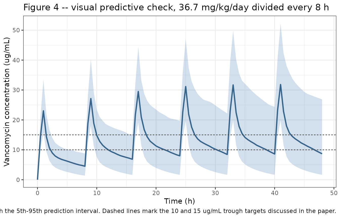
The paper reports that 233 of 347 observed trough concentrations (67%) were below the 10 ug/mL target on the doses actually prescribed, and the Discussion cites a Chinese single-centre figure of 28.17% of patients reaching target. The simulated cohort is checked against that qualitative claim rather than against any single published number, because the trough distribution depends on the covariate distribution assumed above.
# Trough immediately before the sixth dose, which is the sampling time used for
# the paper's own two-patient validation. The sixth dose starts at t = 40 h and
# is infused over 1 h, so nothing has been delivered at t = 40 exactly and the
# concentration there IS the pre-dose trough, independent of record ordering.
troughs <- sim |>
  filter(abs(time - 40) < 1e-6) |>
  summarise(
    n = dplyr::n(),
    median_trough = median(Cc, na.rm = TRUE),
    pct_below_10 = 100 * mean(Cc < 10, na.rm = TRUE)
  )

stopifnot(
  troughs$n == n_subj, # the filter matched every subject
  # The paper's own data put 67% of observed troughs below 10 ug/mL on these
  # doses, and its Discussion is built on target attainment being poor. A
  # simulated majority below target is the reproducible claim; the exact
  # percentage depends on the assumed covariate distribution, so the bound is
  # deliberately wide of any one draw (realised near 70% here).
  troughs$pct_below_10 > 40,
  troughs$pct_below_10 < 95,
  # Structural sanity: a mis-keyed clearance, volume or dose moves the whole
  # trough distribution by tens of percent.
  troughs$median_trough > 2,
  troughs$median_trough < 20
)

troughs |>
  mutate(across(c(median_trough, pct_below_10), ~ sprintf("%.1f", .x))) |>
  dplyr::rename(
    "Subjects" = n,
    "Median trough (ug/mL)" = median_trough,
    "% below 10 ug/mL" = pct_below_10
  ) |>
knitr::kable(caption = "Simulated trough before the sixth dose on 36.7 mg/kg/day divided every 8 h.")| Subjects | Median trough (ug/mL) | % below 10 ug/mL |
|---|---|---|
| 200 | 8.6 | 57.5 |
The paper’s two-patient preliminary validation
Song 2017 closes with a preliminary validation at Southwest Hospital in two pneumonia neonates, reporting for each the birth body weight, the postnatal age at sampling, the prescribed regimen, the measured trough before the sixth dose and the model-predicted trough. Those five facts make the case reproducible here.
validation <- tibble::tribble(
  ~patient, ~bbw, ~pna_d, ~dose_mg, ~observed, ~paper_pred,
  "Patient 1 (S. epidermidis)", 3.9, 23, 35, 4.26, 3.79,
  "Patient 2 (S. aureus)", 4.5, 25, 60, 9.03, 8.73
)

trough_before_6th <- function(bbw, pna_d, dose_mg) {
  ev <- rxode2::et(
    amt = dose_mg, cmt = "central", rate = dose_mg / 1,
    time = seq(0, 32, by = 8)
  ) |>
    rxode2::et(seq(0, 40, by = 0.05))
  dat <- as.data.frame(ev)
  dat$id <- 1L
  dat$WT_BIRTH <- bbw
  dat$PNA <- pna_d / days_per_month
  out <- rxode2::rxSolve(
    rxode2::zeroRe(mod), dat,
    useLinCmt = FALSE, returnType = "data.frame"
  )
  out$Cc[which.min(abs(out$time - 40))]
}

validation <- validation |>
  rowwise() |>
  mutate(pop_pred = trough_before_6th(bbw, pna_d, dose_mg)) |>
  ungroup() |>
  mutate(
    pct_vs_obs = 100 * (pop_pred - observed) / observed,
    pct_vs_paper = 100 * (pop_pred - paper_pred) / paper_pred
  )
#> ℹ parameter labels from comments will be replaced by 'label()'
#> ℹ omega/sigma items treated as zero: 'etalcl'
#> ℹ parameter labels from comments will be replaced by 'label()'
#> ℹ omega/sigma items treated as zero: 'etalcl'

stopifnot(
  nrow(validation) == 2L,
  # The population prediction must at least land in the right order of
  # magnitude for both patients; it does not reproduce the paper's per-patient
  # numbers, for the reason discussed below.
  all(validation$pop_pred > 1 & validation$pop_pred < 20),
  # The two residuals have OPPOSITE signs. That is the signature of per-patient
  # random effects, not of a transcription error, which would bias both the
  # same way. This assertion is the load-bearing part of this section.
  prod(validation$pct_vs_paper) < 0
)

validation |>
  mutate(
    across(c(pop_pred, pct_vs_obs, pct_vs_paper), ~ sprintf("%.2f", .x))
  ) |>
  dplyr::select(patient, bbw, pna_d, dose_mg, observed, paper_pred, pop_pred, pct_vs_paper) |>
  dplyr::rename(
    "Patient" = patient,
    "Birth weight (kg)" = bbw,
    "PNA (days)" = pna_d,
    "Dose (mg q8h)" = dose_mg,
    "Observed trough" = observed,
    "Song 2017 predicted" = paper_pred,
    "This model, typical value" = pop_pred,
    "% vs Song 2017" = pct_vs_paper
  ) |>
knitr::kable(caption = "Song 2017's two-patient preliminary validation (troughs in ug/mL) against the typical-value prediction of the packaged model.")| Patient | Birth weight (kg) | PNA (days) | Dose (mg q8h) | Observed trough | Song 2017 predicted | This model, typical value | % vs Song 2017 |
|---|---|---|---|---|---|---|---|
| Patient 1 (S. epidermidis) | 3.9 | 23 | 35 | 4.26 | 3.79 | 5.45 | 43.78 |
| Patient 2 (S. aureus) | 4.5 | 25 | 60 | 9.03 | 8.73 | 7.27 | -16.75 |
The packaged model’s typical-value trough is above Song 2017’s prediction for patient 1 and below it for patient 2. A transcription error in the structural parameters or the covariate model would bias both patients in the same direction; two residuals of opposite sign instead indicate that the paper’s predictions carry per-patient random effects. That reading is consistent with the paper’s own description of the exercise, in which the predicted trough is compared directly against the therapeutic-drug-monitoring result for the same patient, and both implied deviations are well inside one standard deviation of the reported interindividual variability on clearance (an omega variance of 0.317 is a log-scale standard deviation of 0.563).
This section is therefore reported as a consistency check with a sign-based gate, not as a numerical reproduction of the paper’s two predicted values.
Assumptions and deviations
Interpretation of the reported variability
-
omega-CL= 0.317 is read as a variance, not a standard deviation. The Table 3 legend distinguishes the two scales within a single sentence – “stdev0 = standard deviation; omega-CL = variance of the inter-individual variability of CL” – so the labelling is deliberate rather than incidental, and Phoenix NLME, the tool used, reports its omega block as variances. On this reading the log-scale standard deviation is 0.563 and the apparent coefficient of variation is 61.1%. Were 0.317 instead a standard deviation, the apparent coefficient of variation would be 32.4%. No result in the paper discriminates between the two readings numerically; the legend is the evidence.
Values the paper does not report
- Infusion duration is not stated. Song 2017 records only that vancomycin was given by intravenous infusion, 2 to 4 times daily. The simulations here use a 1 h infusion, the conventional neonatal vancomycin duration. This affects peak concentrations but has almost no effect on the troughs the paper discusses, and none at all on AUC. The closed-form and PKNCA gates above use an intravenous bolus instead, so that the reference side is exact.
- No noncompartmental analysis is published. The paper reports no Cmax, Tmax, AUC or half-life, so the PKNCA comparison above is made against the exact intravenous-bolus identities implied by the paper’s own printed structural parameters, rather than against published noncompartmental values.
- The covariate distributions of the virtual cohort are assumed. Table 1 gives only medians and ranges, not distributional shapes or the correlation between birth weight, postnatal age and current weight. Truncated lognormals matched to the published medians and ranges are used, with current weight grown from birth weight. Only the visual predictive check and the trough summary depend on this assumption; every tight gate in this vignette is deterministic and covariate-grid based.
Canonical-column reparameterisation
-
PNAis supplied in months, not the paper’s days. Song 2017 writes its clearance term as(PNA_days / 29)^0.449. The canonical nlmixr2libPNAcolumn carries months, so the model uses(PNA_months / 0.952772)^0.449with0.952772 = 29 / 30.4375. Numerator and denominator carry the same units factor, so the rescaling is exact and the exponent is unchanged. This follows the same precedent asZhao_2018_omeprazole(days) andBardhi_2026_ampicillin_foal(hours). The covariate-grid gate above is what detects an error here, since the ratio equals 1 at the reference point under either unit. -
The retained size covariate is birth weight, not current
weight. Supplying current body weight in
WT_BIRTHwould misstate every clearance. Current weight was screened by the authors and not retained; it appears incovariatesDataExcludedand is used in this vignette only to size the milligram dose.
Errata and internal inconsistencies in the source
- External-evaluation error units. The Results section reports mean prediction error, mean absolute error and mean squared prediction error as “-0.29 +/- 0.99 ng/mL, 1.388 +/- 0.71 ng/mL and 1.928 +/- 1.665” respectively. Every concentration elsewhere in the paper is in ug/mL, including the assay limit of quantification of 1 ug/mL and the observed median of 9.33 ug/mL, and errors of a nanogram per millilitre would be four orders of magnitude below the assay’s resolution. The unit is read as a typographical slip for ug/mL. Nothing in the model depends on it.
- Mean squared prediction error is reported with a plus-or-minus. A mean squared error is a single non-negative summary, so “1.928 +/- 1.665” is presumably a mean absolute or root-mean-square quantity with its standard deviation. Nothing in the model depends on it.
-
The Table 3 legend calls the covariate exponents “fixed
parameter coefficients”. This is the fixed-effect (THETA) sense
standard in Phoenix NLME, not the held-constant sense: both exponents
are reported with a standard error, a 95% confidence interval and a
bootstrap distribution, so both were estimated. Neither is wrapped in
fixed()in the model file. - The external-evaluation prediction differences are quoted as “-0.2% to 15%” while the two-patient validation quotes prediction errors of 11.0% and 3.32%; the two exercises used different patient sets, so these are not in conflict.
Solver settings
- Every
rxSolve()call in this vignette passesuseLinCmt = FALSE. The model writes its disposition withk12/k21micro-constants, a shape for which rxode2’s default ODE-to-linCmt()auto-conversion has been observed elsewhere in this library to drop the peripheral state silently. It does not do so for this model on rxode2 5.1.8 – with the etas zeroed,useLinCmt = TRUEandFALSEagree onCcto eight significant figures and both retainperipheral1– but the explicit setting is kept as a guard, and the terminal half-life gate above is the check that would go red if a future version did collapse the model, since an AUC gate cannot detect it.