Oral paclitaxel (He 2022)

Model and source

• Citation: He J, Jackson CGCA, Deva S, Hung T, Clarke K, Segelov E, Chao TY, Dai MS, Yeh HT, Ma WW, Kramer D, Chan WK, Kwan R, Cutler D, Zhi J. Population pharmacokinetics for oral paclitaxel in patients with advanced/metastatic solid tumors. CPT Pharmacometrics Syst Pharmacol. 2022;11(7):867-879. doi:10.1002/psp4.12799
• Description: Two-compartment population PK model for oral paclitaxel co-administered with the P-glycoprotein inhibitor encequidar (Oraxol) in adults with advanced or metastatic solid tumors (He 2022). First-order absorption with a fixed lag time, linear elimination, bioavailability fixed at 0.119 for the capsule with a proportional increase for the oral solution, a proportional increase in the central volume for non-Asian patients, and a log-additive residual error. Pooled data from 197 patients in seven studies.
• Article: https://doi.org/10.1002/psp4.12799 (open access)
• Supplement (Appendix S1: Tables S1-S6 including the final NONMEM control stream; Appendix S2: the analysis dataset): https://europepmc.org/article/PMC/PMC9286714

Oraxol is oral paclitaxel given with encequidar, a minimally absorbed P-glycoprotein inhibitor that lets paclitaxel be absorbed from the gut. He 2022 pooled seven studies of oral paclitaxel with encequidar in patients with solid tumors. The final model has two compartments, first-order absorption after a short fixed lag, and linear elimination. Bioavailability is fixed at 0.119 for the capsule, so the clearance and volumes are systemic values given that F. Two covariates were retained: the oral solution’s higher bioavailability, and a larger central volume in non-Asian patients.

Population

The model was developed from 197 adults with advanced or metastatic solid tumors (gastric cancer, metastatic breast cancer, lung cancer and others) enrolled in seven studies in the Republic of Korea, the United States, New Zealand, Australia and Taiwan (He 2022 Table S1). They contributed 4322 plasma paclitaxel concentrations. Mean age was 59.6 years (range 32-81), mean weight 67.2 kg (38-139) and mean body surface area 1.73 m^2 (1.29-2.46). 52.3% were female; 55.8% were Asian and 41.1% Caucasian. 59.9% had mild or moderate renal impairment and 10.2% had (mostly mild) hepatic impairment (He 2022 Table 1). Oral doses ranged from 60 to 420 mg/m^2. The two bioavailability studies, and the phase III regimen, used 205 mg/m^2 once daily on days 1-3 of each week. 92.4% of patients took capsules; the other 15, all in the first study, took the intravenous paclitaxel solution by mouth.

The same information is available programmatically via readModelDb("He_2022_paclitaxel")()$population.

Source trace

Every ini() value carries an in-file comment pointing to its source in inst/modeldb/specificDrugs/He_2022_paclitaxel.R. The table below collects them.

Equation / parameter	Value	Source location
lcl (CL)	log(33.7) L/h	Table 2; Table S4
lvc (V2, Asian)	log(50.7) L	Table 2; Table S4
lq (Q)	log(40.6) L/h	Table 2; Table S4
lvp (V3)	log(855) L	Table 2; Table S4
lka (KA)	log(0.724) 1/h	Table 2; Table S4
ltlag (ALAG1)	fixed(log(0.215)) h	Table 2 (fixed); Table S6 THETA(7)
lfdepot (F1, capsule)	fixed(log(0.119))	Table 2 (fixed); Table S6 THETA(6)
e_race_nonasian_vc	0.696	Table 2 ‘Race on V2 (proportional)’; Table S6 THETA(8)
e_form_solution_fdepot	0.895	Table 2 ‘Formulation on F1 (proportional)’; Table S6 THETA(9)
etalcl	0.1118	Table 2 ‘ETA CL’ 34.4 CV%, as log(CV^2 + 1)
etalvc	1.4104	Table 2 ‘ETA V2’ 176 CV%, as log(CV^2 + 1)
etalfdepot	0.2073	Table S4 ‘BSV on F1’ 48.0 CV%, as log(CV^2 + 1); Table S6 eta6 on F1
expSd	sqrt(0.208) = 0.4561	Table 2 ‘Log additive’ 0.208 (SIGMA variance); Table S6 Y = LOG(F) + ERR(1)
vc <- ... * (1 + e * (1 - RACE_ASIAN))	n/a	Table S6 TVV2 = THETA(2)*(1 + THETA(8)*RACB), RACB = non-Asian
fdepot <- ... * (1 + e * FORM_SOLUTION)	n/a	Table S6 TVF1 = THETA(6)*(1 + THETA(9)*(2-FORM)), FORM 1 = solution
ODEs, alag(depot), f(depot)	n/a	Table S6 ADVAN4 TRANS4, Figure 1
Cc <- central / vc * 1000	n/a	Table S6 S2 = V2/1000 (dose in mg, concentration in ng/mL)

mod <- readModelDb("He_2022_paclitaxel")
mod_typical <- mod |> rxode2::zeroRe()
#> ℹ parameter labels from comments will be replaced by 'label()'

Typical-value checks against printed values

The Results section prints two derived typical values: the non-Asian central volume, 50.7 x (1 + 0.696) = 86.0 L, and the oral-solution bioavailability, 0.226. Both come out of the model’s own model() block.

ev_one <- rxode2::et(amt = 100, cmt = "depot") |>
  rxode2::et(c(0, 1, 2))
derived <- dplyr::bind_rows(
  lapply(
    list(
      c(RACE_ASIAN = 1, FORM_SOLUTION = 0),
      c(RACE_ASIAN = 0, FORM_SOLUTION = 0),
      c(RACE_ASIAN = 1, FORM_SOLUTION = 1)
    ),
    function(cv) {
      s <- rxode2::rxSolve(mod_typical, ev_one, params = cv)
      data.frame(
        RACE_ASIAN = cv[["RACE_ASIAN"]],
        FORM_SOLUTION = cv[["FORM_SOLUTION"]],
        vc = s$vc[1],
        fdepot = s$fdepot[1]
      )
    }
  )
)
#> ℹ omega/sigma items treated as zero: 'etalcl', 'etalvc', 'etalfdepot'
#> ℹ omega/sigma items treated as zero: 'etalcl', 'etalvc', 'etalfdepot'
#> ℹ omega/sigma items treated as zero: 'etalcl', 'etalvc', 'etalfdepot'
knitr::kable(derived, digits = 4, caption = "Typical V2 (L) and F1 by covariate level.")

Typical V2 (L) and F1 by covariate level.

RACE_ASIAN	FORM_SOLUTION	vc	fdepot
1	0	50.7000	0.1190
0	0	85.9872	0.1190
1	1	50.7000	0.2255

stopifnot(
  # Printed '50.7 x (1 + 0.696) = 86.0 L' for non-Asian patients.
  abs(derived$vc[2] - 86.0) < 0.05,
  abs(derived$vc[1] - 50.7) < 1e-8,
  # Printed 'bioavailability estimated to be 0.226' for the oral solution.
  abs(derived$fdepot[3] - 0.226) < 0.0005,
  abs(derived$fdepot[1] - 0.119) < 1e-8
)

Because the model is linear, the total AUC after a capsule dose is F x Dose / CL exactly. A typical-value solve recovers that identity. The Introduction also states that 205 mg/m^2 by mouth on three consecutive days gives a systemic AUC similar to 80 mg/m^2 intravenous paclitaxel. Under this model the ratio is 3 x 0.119 x 205 / 80 = 0.915, whatever the clearance. The intravenous dose is given straight into central; F1 applies to depot only.

bsa_ref <- 1.73
# Fine grid over the fast distribution phase (alpha ~ 1.5 1/h), coarse tail.
auc_grid <- sort(unique(c(seq(0, 200, by = 0.02), seq(200, 3000, by = 0.5))))
ev_oral <- rxode2::et(
  amt = 205 * bsa_ref, cmt = "depot", time = c(0, 24, 48)
) |>
  rxode2::et(auc_grid)
ev_iv <- rxode2::et(
  amt = 80 * bsa_ref, cmt = "central", time = 0, dur = 1
) |>
  rxode2::et(auc_grid)
cov_ref <- c(RACE_ASIAN = 1, FORM_SOLUTION = 0)
s_oral <- as.data.frame(rxode2::rxSolve(
  mod_typical, ev_oral,
  params = cov_ref, rtol = 1e-10, atol = 1e-12
))
#> ℹ omega/sigma items treated as zero: 'etalcl', 'etalvc', 'etalfdepot'
s_iv <- as.data.frame(rxode2::rxSolve(
  mod_typical, ev_iv,
  params = cov_ref, rtol = 1e-10, atol = 1e-12
))
#> ℹ omega/sigma items treated as zero: 'etalcl', 'etalvc', 'etalfdepot'

trap <- function(t, y) sum(diff(t) * (head(y, -1) + tail(y, -1)) / 2)
auc_oral <- trap(s_oral$time, s_oral$Cc)
auc_iv <- trap(s_iv$time, s_iv$Cc)
auc_oral_cf <- 3 * 0.119 * 205 * bsa_ref / 33.7 * 1000
auc_iv_cf <- 80 * bsa_ref / 33.7 * 1000
data.frame(
  regimen = c("Oral 205 mg/m^2 QD x 3 (capsule)", "IV 80 mg/m^2, 1-h infusion"),
  auc_solver = c(auc_oral, auc_iv),
  auc_closed_form = c(auc_oral_cf, auc_iv_cf)
) |>
  dplyr::rename(
    "Regimen (BSA 1.73 m^2)" = regimen,
    "AUC0-3000h, solver (ng*h/mL)" = auc_solver,
    "F x Dose / CL (ng*h/mL)" = auc_closed_form
  ) |>
  knitr::kable(digits = 0)

Regimen (BSA 1.73 m^2)	AUC0-3000h, solver (ng*h/mL)	F x Dose / CL (ng*h/mL)
Oral 205 mg/m^2 QD x 3 (capsule)	3757	3757
IV 80 mg/m^2, 1-h infusion	4107	4107

stopifnot(
  # Linear trapezoid on the 0.02 h grid: the error scales with the grid
  # spacing squared (0.4% on a 0.5 h grid, so < 1e-4 here); the 3000 h
  # window leaves < 1e-6 of the AUC unsampled.
  abs(auc_oral / auc_oral_cf - 1) < 1e-3,
  abs(auc_iv / auc_iv_cf - 1) < 1e-3,
  # Introduction: oral 205 mg/m^2 x 3 days 'similar to' 80 mg/m^2 IV.
  abs(auc_oral / auc_iv - 3 * 0.119 * 205 / 80) < 1e-3
)

Virtual cohort

He 2022 simulated 1000 capsule patients (500 Asian, 500 non-Asian) on the phase III regimen: 205 mg/m^2 once daily on days 1-3 of each week for three weeks. The cohort below has 200 patients, half of them Asian. Body surface area is drawn from a normal distribution with the Table 1 mean and SD, then truncated to the Table 1 range. The dose is 205 mg/m^2 times each patient’s body surface area.

rxode2::rxSetSeed(20220714)
set.seed(20220714)
n_sub <- 200L
dose_times <- c(0, 24, 48, 168, 192, 216, 336, 360, 384)
obs_times <- seq(0, 504, by = 0.5)

subjects <- tibble::tibble(
  id = seq_len(n_sub),
  RACE_ASIAN = rep(c(1L, 0L), length.out = n_sub),
  FORM_SOLUTION = 0L,
  BSA = pmin(pmax(rnorm(n_sub, 1.73, 0.23), 1.29), 2.46)
) |>
  dplyr::mutate(race = ifelse(RACE_ASIAN == 1, "Asian", "Non-Asian"))

events <- dplyr::bind_rows(
  subjects |>
    tidyr::crossing(time = dose_times) |>
    dplyr::mutate(evid = 1L, amt = 205 * BSA, cmt = "depot"),
  subjects |>
    tidyr::crossing(time = obs_times) |>
    dplyr::mutate(evid = 0L, amt = 0, cmt = "central")
) |>
  dplyr::arrange(id, time, dplyr::desc(evid)) |>
  dplyr::mutate(treatment = "Oral 205 mg/m^2 QD x 3 weekly")

stopifnot(
  length(unique(events$id)) == n_sub,
  sum(events$evid == 1) == n_sub * length(dose_times)
)

Simulation

sim <- rxode2::rxSolve(
  mod,
  events = events,
  keep = c("treatment", "race", "BSA")
) |>
  as.data.frame()
#> ℹ parameter labels from comments will be replaced by 'label()'
# Paclitaxel 0.05 umol/L, the T > 0.05 uM threshold of Table S5
# (molar mass 853.9 g/mol); the paper's figures round it to 40 ng/mL.
c_thr <- 0.05 * 853.9

Replicate published figures

# Replicates Figure 4a of He 2022: individual simulated concentrations and
# mean + SD on the paper's sampling schedule (pre-dose, 1-4 h after each dose,
# then daily), with the 40 and 10 ng/mL reference lines. Values below the
# 2.5 ng/mL LLOQ are set to missing, as in the paper.
wk <- c(0, 1, 2, 3, 4, 24, 25, 26, 27, 28, 48, 49, 50, 51, 52, 72, 96, 120, 144)
fig_times <- sort(unique(c(wk, wk + 168, wk + 336, 504)))
fig_dat <- sim |>
  dplyr::filter(time %in% fig_times) |>
  dplyr::mutate(Cc = ifelse(Cc < 2.5, NA_real_, Cc))
fig_mean <- fig_dat |>
  dplyr::group_by(time) |>
  dplyr::summarise(
    mean = mean(Cc, na.rm = TRUE),
    sd = sd(Cc, na.rm = TRUE),
    .groups = "drop"
  ) |>
  # Pre-dose at time 0 every value is below the LLOQ, so there is no mean.
  dplyr::filter(is.finite(mean))
ggplot(fig_dat, aes(time, Cc)) +
  geom_point(size = 0.4, alpha = 0.3, na.rm = TRUE) +
  geom_line(data = fig_mean, aes(time, mean), colour = "red") +
  geom_errorbar(
    data = fig_mean,
    aes(x = time, ymin = mean, ymax = mean + sd),
    inherit.aes = FALSE, colour = "red", width = 4
  ) +
  geom_hline(yintercept = c(40, 10), colour = "blue", linetype = "dashed") +
  scale_y_log10() +
  scale_x_continuous(breaks = seq(0, 504, by = 168)) +
  labs(
    x = "Time (h)", y = "Paclitaxel concentration (ng/mL)",
    title = "Oral paclitaxel 205 mg/m^2 QD x 3 for 3 weeks",
    caption = "Replicates Figure 4a of He 2022."
  )

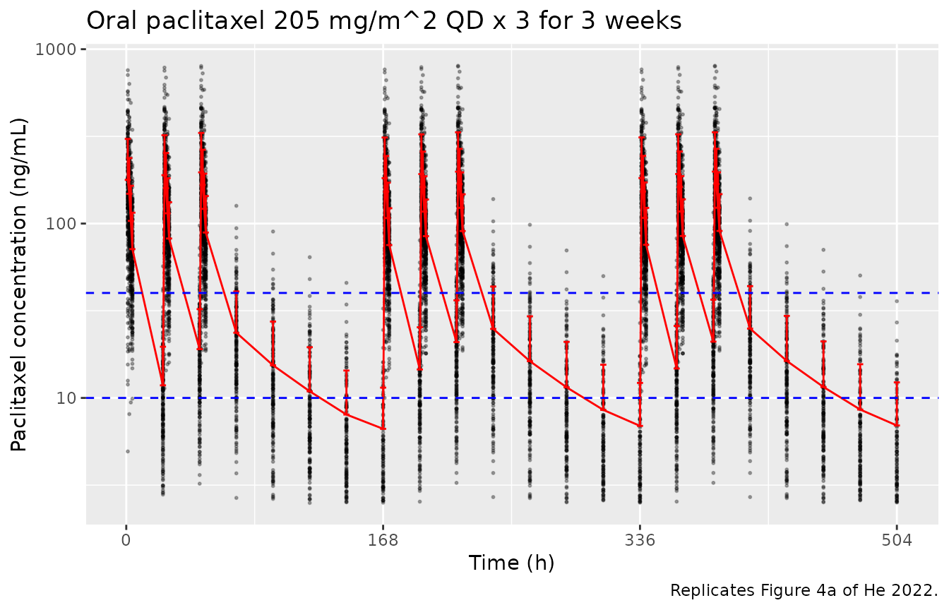
The simulated profile has the shape of Figure 4a. Mean concentrations peak at about 180-200 ng/mL one hour after each dose and fall to a mean of about 15-25 ng/mL by the next dose. Between dosing blocks they decline to a mean of about 7 ng/mL (quantifiable values only) before the next week’s first dose. The mean profile repeats from week to week with no visible accumulation, which matches the paper’s statement that exposure was reproducible over weeks 1-4 (Figure S2).

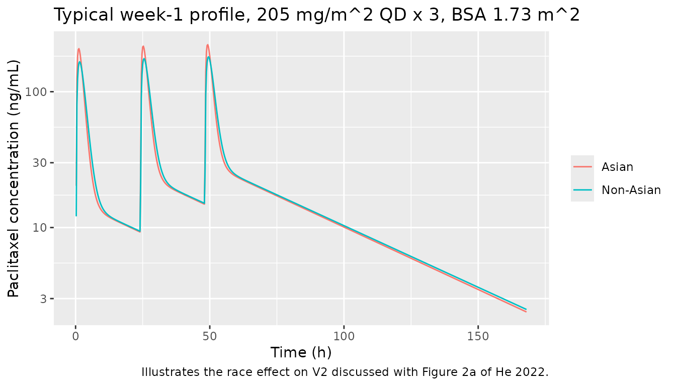
# Typical profile by race (the only covariate on disposition): the larger
# non-Asian V2 lowers the peak and leaves the AUC unchanged.
ev_wk1 <- rxode2::et(amt = 205 * 1.73, cmt = "depot", time = c(0, 24, 48)) |>
  rxode2::et(seq(0, 168, by = 0.25))
typ <- dplyr::bind_rows(
  as.data.frame(rxode2::rxSolve(mod_typical, ev_wk1,
    params = c(RACE_ASIAN = 1, FORM_SOLUTION = 0)
  )) |> dplyr::mutate(race = "Asian"),
  as.data.frame(rxode2::rxSolve(mod_typical, ev_wk1,
    params = c(RACE_ASIAN = 0, FORM_SOLUTION = 0)
  )) |> dplyr::mutate(race = "Non-Asian")
) |>
  # Drop the pre-absorption rows (Cc = 0 before the lag) for the log axis.
  dplyr::filter(time >= 0.25)
#> ℹ omega/sigma items treated as zero: 'etalcl', 'etalvc', 'etalfdepot'
#> ℹ omega/sigma items treated as zero: 'etalcl', 'etalvc', 'etalfdepot'
ggplot(typ, aes(time, Cc, colour = race)) +
  geom_line() +
  scale_y_log10() +
  labs(
    x = "Time (h)", y = "Paclitaxel concentration (ng/mL)", colour = NULL,
    title = "Typical week-1 profile, 205 mg/m^2 QD x 3, BSA 1.73 m^2",
    caption = "Illustrates the race effect on V2 discussed with Figure 2a of He 2022."
  )

PKNCA validation

sim_nca <- sim |>
  dplyr::filter(!is.na(Cc)) |>
  dplyr::select(id, time, Cc, treatment)
sim_nca <- dplyr::bind_rows(
  sim_nca,
  sim_nca |> dplyr::distinct(id, treatment) |> dplyr::mutate(time = 0, Cc = 0)
) |>
  dplyr::distinct(id, treatment, time, .keep_all = TRUE) |>
  dplyr::arrange(id, treatment, time)

conc_obj <- PKNCA::PKNCAconc(sim_nca, Cc ~ time | treatment + id)
dose_df <- events |>
  dplyr::filter(evid == 1) |>
  dplyr::select(id, time, amt, treatment)
dose_obj <- PKNCA::PKNCAdose(dose_df, amt ~ time | treatment + id)

intervals <- data.frame(
  start = 0,
  end = 504,
  auclast = TRUE,
  cmax = TRUE,
  time_above = TRUE,
  # PKNCA reads the time_above threshold from this interval column.
  conc_above = c_thr
)
nca_data <- PKNCA::PKNCAdata(conc_obj, dose_obj, intervals = intervals)
nca_res <- PKNCA::pk.nca(nca_data)
summary(nca_res)
#>  start end                     treatment   N      auclast       cmax
#>      0 504 Oral 205 mg/m^2 QD x 3 weekly 200 11400 [63.2] 180 [69.1]
#>   time_above
#>  75.9 [72.6]
#> 
#> Caption: auclast, cmax: geometric mean and geometric coefficient of variation; time_above: arithmetic mean and standard deviation; N: number of subjects

Comparison against published NCA

Table S5 reports NCA of the paper’s own simulation of this regimen. The comparison uses its medians.

published <- tibble::tribble(
  ~treatment, ~auclast, ~cmax, ~time_above,
  "Oral 205 mg/m^2 QD x 3 weekly", 14168, 268, 93
)
# ncaParamLabel() has no friendly label for 'time_above' and warns; muffle
# only that warning, so any other one still surfaces.
cmp <- withCallingHandlers(
  nlmixr2lib::ncaComparisonTable(
    simulated = nca_res,
    reference = published,
    by = "treatment",
    units = c(auclast = "ng*h/mL", cmax = "ng/mL", time_above = "h"),
    tolerance_pct = 20
  ),
  warning = function(w) {
    if (grepl("time_above", conditionMessage(w))) {
      invokeRestart("muffleWarning")
    }
  }
)
knitr::kable(
  cmp,
  caption = paste(
    "Simulated vs. published (Table S5 median) NCA over 0-504 h.",
    "* differs from reference by >20%."
  )
)

Simulated vs. published (Table S5 median) NCA over 0-504 h. * differs from reference by >20%.

NCA parameter	treatment	Reference	Simulated	% diff
Cmax (ng/mL)	Oral 205 mg/m^2 QD x 3 weekly	268	182	-32.2%*
AUClast (ng*h/mL)	Oral 205 mg/m^2 QD x 3 weekly	14200	11800	-17.0%
time_above (h)	Oral 205 mg/m^2 QD x 3 weekly	93	50.4	-45.9%*

The simulated medians come out below Table S5: AUC0-504 by about a sixth, Cmax by about a third, and time above 0.05 umol/L by about half. This gap does not point to a transcription error. The maintainers evaluated the published model on the paper’s own analysis dataset (Appendix S2), and its objective function matches Table 2 (see Assumptions and deviations below). Instead, the Table S5 numbers depend on how the paper’s simulation was done, which Methods describes only partly:

• NCA was run in Phoenix WinNonlin on concentrations simulated at the sparse clinical schedule (pre-dose, 1-4 h after each dose, then every 24 h), with values below 2.5 ng/mL set to missing (Figure 4 legend). Trapezoids across the 4-24 h gaps after each peak overstate the AUC. On that schedule, this model’s median AUC0-504 rises to roughly 16,000-18,000 ng*h/mL, depending on the trapezoid rule, which brackets the published 14,168.
• The published Cmax and T > 0.05 uM likely include residual error and use that sparse grid. The CV of the Table S5 AUC (37%) is also smaller than the 34.4% CL and 48.0% F1 variabilities combine to give (about 60%). This suggests the paper’s simulation did not carry the full IIV structure described in Table S4. One possibility is the Table 2 row that labels the 48.0% IIV as “ETA Q”.
• N in Table S5 (264 oral, 135 intravenous) matches neither the stated 1000 simulated patients nor this cohort. The covariates and doses used are not given.

The intravenous arm of Table S5 (175 mg/m^2 over 3 h, mean AUC0-504 16,502 ngh/mL) cannot come from this model either. With the linear CL = 33.7 L/h, a 175 mg/m^2 dose at 1.73 m^2 gives AUC = Dose / CL = 8984 ngh/mL. That is about half the published value, in line with the saturable clearance of intravenous paclitaxel at that dose, which the oral model does not describe. The paper does not say which model it used for the intravenous simulation, so that arm is not reproduced here.

For these reasons the vignette gates on the model-level identities above, not on Table S5.

Assumptions and deviations

• IIV on F1, not on Q. Table 2 labels the third IIV row “ETA Q (CV%) 48.0”. Table S4 calls the same row “BSV on F1”, and the final control stream (Table S6) estimates eta6 on F1 with the eta on Q fixed to 0. The model places this IIV on F1. Evaluating the objective function on the Appendix S2 data confirms it: OFV -1278.7 with the IIV on F1, against -926.8 with it on Q.

• Variance scales. Table 2 gives the IIV as CV% and the residual error as “Log additive 0.208”. The maintainers evaluated the final model, with parameters held at the published values, on the Appendix S2 analysis dataset restricted to the 197 patients and 4322 observations of the analysis (rollover-patient records and the eighth, later study excluded; BLQ records dropped as in Table S6). The four readings of the scales give these objective function values:

  IIV as	Residual 0.208 as	OFV
  log(CV^2 + 1)	variance (SD 0.456)	-1278.7
  (CV/100)^2	variance (SD 0.456)	-1246.6
  log(CV^2 + 1)	SD	7206.8
  (CV/100)^2	SD	7218.0

  Only the first reading matches the printed OFV of 1279.4 to within 1 unit in magnitude. The model therefore uses omega^2 = log(CV^2 + 1) and a log-scale residual SD of sqrt(0.208). Table 2 prints the OFV without a minus sign. For log-transformed data with a log-scale residual variance of 0.208 the OFV is negative, so the printed value is taken to be missing its sign. The dataset is not redistributed with the package. Its licence (CC BY-NC-ND) does not allow it, so this check is not re-run here.

• Race coding. The control stream’s RACB is 1 for every non-Asian race code (Caucasian, African American, American Indian, Native Hawaiian or Other Pacific Islander) and 0 for Asian. The model uses 1 - RACE_ASIAN in its place. The Appendix S2 dataset confirms that RACE = 0 is Asian (110 patients, matching Table 1).

• Formulation. FORM_SOLUTION = 2 - FORM, with source FORM 1 = solution and 2 = capsule (Figure 3 legend). Use FORM_SOLUTION = 0 for the marketed capsule.

• Encequidar. Every observation in the analysis came from paclitaxel given with encequidar. Encequidar dose and timing were screened on F1 (Table S3) and not retained. The model does not apply to oral paclitaxel without encequidar.

• Food. 97% of patients were dosed fasted, and the paper draws no conclusion on food. The model describes fasted dosing.

• Virtual cohort. Body surface area was drawn from a truncated normal distribution using the Table 1 mean, SD and range. Doses were not rounded to capsule strengths.

• Errata. No correction notice for this article was found in Europe PMC as of 2026-10-02.