Rifapentine and isoniazid, whole vs suspended tablets (Janssen 2025)
Source:vignettes/articles/Janssen_2025_rifapentine_isoniazid.Rmd
Janssen_2025_rifapentine_isoniazid.RmdModel and source
Janssen et al. (2025) gave 24 adults on once-weekly rifapentine/isoniazid (3HP) tuberculosis preventive therapy 900 mg of each drug, either as whole tablets or as tablets crushed and suspended in water, and fitted one population PK model per drug. Both are packaged:
-
Janssen_2025_rifapentine: One-compartment population PK model for oral rifapentine in South African adults on once-weekly rifapentine/isoniazid (3HP) tuberculosis preventive therapy (Janssen 2025). Absorption is a Savic transit chain (4 transit compartments, absorption rate equal to the transit rate) whose mean transit time is shortened when the tablets are suspended in water; IOV on bioavailability and MTT is correlated and the MTT IOV is smaller after suspended tablets. Parameters are for a 900 mg dose. -
Janssen_2025_isoniazid: Two-compartment population PK model for oral isoniazid in South African adults on once-weekly rifapentine/isoniazid (3HP) tuberculosis preventive therapy (Janssen 2025). A two-class mixture separates fast/intermediate from slow acetylators on CL/F (supplied here as NAT2_SLOW); CL, Q, V and Vp scale allometrically with fat-free mass (reference 45 kg). Absorption is a Savic transit chain (5 transit compartments, absorption rate equal to the transit rate) whose mean transit time is shortened when the tablets are suspended in water; IOV on bioavailability and MTT, with smaller MTT IOV after suspended tablets. - Citation: Janssen S, Vongjarudech T, Karlsson MO, Upton CM, Garcia-Prats AJ, Diacon AH, Wiesner L, Sachs T, van der Laan LE, Salazar-Austin N, Hesseling AC, Svensson EM. Bridging to Paediatric Dosing: Relative Bioavailability of Suspended Rifapentine and Isoniazid in an Open-Label Randomized Trial in Adults on Tuberculosis Preventive Therapy. Clin Pharmacokinet. 2025;64(12):1885. doi:10.1007/s40262-025-01576-3
- Article: https://doi.org/10.1007/s40262-025-01576-3
The NONMEM control streams of both final models are in the paper’s Electronic Supplementary Material (ESM 2 for rifapentine, ESM 3 for isoniazid) and were used to confirm every structural element.
Population
The study was an open-label randomised crossover at one site in Cape Town, South Africa. Adults aged 18-55 years weighing 40-90 kg, with a positive tuberculosis infection test after recent household contact with drug-susceptible pulmonary TB, were randomised 1:1:1 to receive two of three products (two generic rifapentine/isoniazid 300/300 mg fixed-dose combinations, or standalone 300 mg tablets of each drug), each once whole and once suspended, over the first four weekly doses. Doses were taken 30 min after a standard 670 kcal breakfast. Of the 24 analysed participants, 83.3% were female and 91.7% of mixed race; median age 37.5 years, weight 61.1 kg and fat-free mass 38.6 kg (Table 1). The analysis used 838 rifapentine and 707 isoniazid concentrations; BLQ samples were omitted.
The same information is available programmatically via
readModelDb("Janssen_2025_rifapentine")()$population.
Source trace
| Equation / parameter | Rifapentine | Isoniazid | Source location |
|---|---|---|---|
| Structure | 1-compartment | 2-compartment | Results, PopPK paragraph; ESM 2 / ESM 3 $DES
|
Transit chain NN,
ka = ktr = (NN+1)/MTT
|
4 | 5 | ESM 2 / ESM 3 $PK (NN, KTR,
KA) |
lcl / lcl_nonslow (L/h) |
1.03 | 23.3 (fast/intermediate) | Table 2, CL/F |
lcl_slow (L/h) |
– | 9.5 | Table 2, CL slow/F |
| Fraction fast/intermediate acetylators | – | 65.9% | Table 2; ESM 3 $MIX
|
lvc (L) |
26.56 | 59.6 | Table 2, V/F |
lq (L/h) |
– | 1.26 | Table 2, Q/F |
lvp (L) |
– | 56.7 | Table 2, Vp/F |
lmtt (h) |
2.75 | 1.4 | ESM 2 $THETA TVMTT (see Assumptions); Table 2, MTT |
lfdepot |
1 (fixed) | 1 (fixed) | Table 2, F |
FFM allometry, (FFM/45)^x
|
– | 0.75 on CL, Q; 1 on V, Vp (fixed) | Table 2 footnote b; ESM 3 FCL, FV
|
e_susp_mtt |
-0.222 | -0.35 | Table 2, effect of suspension on MTT |
e_susp_iovmtt |
-0.458 | -0.629 | Table 2, effect of suspension on MTT variation; ESM 2 / ESM 3
MTT for OFORM = 2
|
| IIV CL (%CV) | 19.9 | 17.4 | Table 2 |
| IIV F (%CV) | 17.3 | 18.1 | Table 2 |
| IOV F (%CV) | 12.2 | 7.1 | Table 2 |
| IOV MTT (%CV) | 39.2 | 40.8 | Table 2 |
| IOV F-MTT correlation | 0.37 | none | Table 2; ESM 2 $OMEGA BLOCK(2), ESM 3
BLOCK(1)
|
propSd |
0.08 | 0.208 | Table 2, proportional error |
addSd (mg/L) |
1.7 | 0.11 | Table 2, additive error |
Variances are omega^2 = log(1 + CV^2), the inverse of
Table 2 footnote c.
Virtual cohort
Each simulated subject receives one 900 mg dose of each drug at occasion 1, either whole or suspended (150 subjects per formulation). Fat-free mass is log-normal around the Table 1 median of 38.6 kg with its interquartile range (34.5-42.8 kg); the isoniazid acetylator class is drawn with the fitted fast/intermediate probability of 0.659.
set.seed(20251)
n_per_arm <- 150
grid_fine <- sort(unique(c(seq(0, 12, by = 0.25), 13:48)))
grid_protocol <- c(0, 1, 2, 3, 4, 5, 6, 8, 24, 48)
grid <- sort(unique(c(grid_fine, grid_protocol)))

make_cohort <- function(n, susp, id_offset) {
  subj <- tibble(
    id = id_offset + seq_len(n),
    FORM_SUSPENSION = susp,
    FFM = exp(rnorm(n, log(38.6), (log(42.8) - log(34.5)) / 1.349)),
    NAT2_SLOW = rbinom(n, 1, 1 - 0.659)
  )
  dose <- subj |> mutate(time = 0, evid = 1L, amt = 900, cmt = "depot")
  obs <- subj |>
    tidyr::crossing(time = grid) |>
    mutate(evid = 0L, amt = 0, cmt = "central")
  bind_rows(dose, obs) |>
    mutate(OCC = 1L, form = ifelse(susp == 1, "Suspension", "Whole tablet")) |>
    arrange(id, time, desc(evid))
}

events <- bind_rows(
  make_cohort(n_per_arm, 0, id_offset = 0L),
  make_cohort(n_per_arm, 1, id_offset = n_per_arm)
)
stopifnot(!anyDuplicated(unique(events[, c("id", "time", "evid")])))
Simulation
mod_rpt <- readModelDb("Janssen_2025_rifapentine")
mod_inh <- readModelDb("Janssen_2025_isoniazid")

rxode2::rxSetSeed(20251)
sim_rpt <- rxode2::rxSolve(mod_rpt, events = events, keep = c("form")) |>
  as.data.frame() |>
  mutate(drug = "Rifapentine")
#> ℹ parameter labels from comments will be replaced by 'label()'
#> Warning: some etas defaulted to non-mu referenced, possible parsing error: etaiov_lfdepot_1, etaiov_lmtt_1, etaiov_lfdepot_2, etaiov_lmtt_2, etaiov_lfdepot_3, etaiov_lmtt_3, etaiov_lfdepot_4, etaiov_lmtt_4
#> as a work-around try putting the mu-referenced expression on a simple line
sim_inh <- rxode2::rxSolve(
  mod_inh,
  events = events,
  keep = c("form", "NAT2_SLOW")
) |>
  as.data.frame() |>
  mutate(
    drug = "Isoniazid",
    acetylator = ifelse(NAT2_SLOW == 1, "Slow", "Fast/intermediate")
  )
#> ℹ parameter labels from comments will be replaced by 'label()'
#> Warning: some etas defaulted to non-mu referenced, possible parsing error: etaiov_lfdepot_1, etaiov_lfdepot_2, etaiov_lfdepot_3, etaiov_lfdepot_4, etaiov_lmtt_1, etaiov_lmtt_2, etaiov_lmtt_3, etaiov_lmtt_4
#> as a work-around try putting the mu-referenced expression on a simple line
Mass balance of the transit chain
The packaged models write the published Savic analytical transit
input as an explicit chain of first-order compartments. With the random
effects removed, the area under the curve of a single dose must equal
F * dose / CL, which checks that no dose is lost or
duplicated along the chain.
t_mb <- seq(0, 600, by = 0.05)
ev_mb <- tibble(
  id = 1L, time = c(0, t_mb),
  evid = c(1L, rep(0L, length(t_mb))), amt = c(900, rep(0, length(t_mb))),
  cmt = c("depot", rep("central", length(t_mb))),
  FORM_SUSPENSION = 0, FFM = 45, NAT2_SLOW = 0, OCC = 1L
)
auc_typ <- function(mod) {
  s <- rxode2::rxSolve(rxode2::zeroRe(mod), events = ev_mb, atol = 1e-10, rtol = 1e-10)
  PKNCA::pk.calc.auc.last(conc = s$Cc, time = s$time, method = "linear")
}
mb <- tibble(
  drug = c("Rifapentine", "Isoniazid"),
  auc_solved = c(auc_typ(mod_rpt), auc_typ(mod_inh)),
  auc_expected = c(900 / 1.03, 900 / 23.3)
) |>
  mutate(pct_diff = 100 * (auc_solved / auc_expected - 1))
#> ℹ parameter labels from comments will be replaced by 'label()'
#> Warning: some etas defaulted to non-mu referenced, possible parsing error: etaiov_lfdepot_1, etaiov_lmtt_1, etaiov_lfdepot_2, etaiov_lmtt_2, etaiov_lfdepot_3, etaiov_lmtt_3, etaiov_lfdepot_4, etaiov_lmtt_4
#> as a work-around try putting the mu-referenced expression on a simple line
#> Warning: some etas defaulted to non-mu referenced, possible parsing error: etaiov_lfdepot_1, etaiov_lmtt_1, etaiov_lfdepot_2, etaiov_lmtt_2, etaiov_lfdepot_3, etaiov_lmtt_3, etaiov_lfdepot_4, etaiov_lmtt_4
#> as a work-around try putting the mu-referenced expression on a simple line
#> ℹ omega/sigma items treated as zero: 'etalcl', 'etalfdepot', 'etaiov_lfdepot_1', 'etaiov_lmtt_1', 'etaiov_lfdepot_2', 'etaiov_lmtt_2', 'etaiov_lfdepot_3', 'etaiov_lmtt_3', 'etaiov_lfdepot_4', 'etaiov_lmtt_4'
#> ℹ parameter labels from comments will be replaced by 'label()'
#> Warning: some etas defaulted to non-mu referenced, possible parsing error: etaiov_lfdepot_1, etaiov_lfdepot_2, etaiov_lfdepot_3, etaiov_lfdepot_4, etaiov_lmtt_1, etaiov_lmtt_2, etaiov_lmtt_3, etaiov_lmtt_4
#> as a work-around try putting the mu-referenced expression on a simple line
#> Warning: some etas defaulted to non-mu referenced, possible parsing error: etaiov_lfdepot_1, etaiov_lfdepot_2, etaiov_lfdepot_3, etaiov_lfdepot_4, etaiov_lmtt_1, etaiov_lmtt_2, etaiov_lmtt_3, etaiov_lmtt_4
#> as a work-around try putting the mu-referenced expression on a simple line
#> ℹ omega/sigma items treated as zero: 'etalcl', 'etalfdepot', 'etaiov_lfdepot_1', 'etaiov_lfdepot_2', 'etaiov_lfdepot_3', 'etaiov_lfdepot_4', 'etaiov_lmtt_1', 'etaiov_lmtt_2', 'etaiov_lmtt_3', 'etaiov_lmtt_4'
knitr::kable(mb, digits = c(0, 2, 2, 3), caption = "Typical-value AUC0-600 vs F * dose / CL.")| drug | auc_solved | auc_expected | pct_diff |
|---|---|---|---|
| Rifapentine | 873.79 | 873.79 | 0 |
| Isoniazid | 38.63 | 38.63 | 0 |
Replicate published figures
vpc <- function(sim, ...) {
  sim |>
    group_by(time, form, ...) |>
    summarise(
      Q05 = quantile(Cc, 0.05), Q50 = quantile(Cc, 0.50), Q95 = quantile(Cc, 0.95),
      .groups = "drop"
    )
}
vpc(sim_rpt) |>
  ggplot(aes(time, Q50)) +
  geom_ribbon(aes(ymin = Q05, ymax = Q95), alpha = 0.25, fill = "steelblue") +
  geom_line() +
  facet_wrap(~form) +
  labs(
    x = "Time after dose (h)", y = "Rifapentine concentration (mg/L)",
    title = "Rifapentine, 900 mg: simulated median and 90% interval",
    caption = "Replicates Figure 3 of Janssen 2025 (pooled over products)."
  )
vpc(filter(sim_inh, time <= 24), acetylator) |>
  ggplot(aes(time, Q50)) +
  geom_ribbon(aes(ymin = Q05, ymax = Q95), alpha = 0.25, fill = "darkorange") +
  geom_line() +
  facet_grid(acetylator ~ form) +
  labs(
    x = "Time after dose (h)", y = "Isoniazid concentration (mg/L)",
    title = "Isoniazid, 900 mg: simulated median and 90% interval",
    caption = "Replicates Figure 4A (fast/intermediate) and 4B (slow) of Janssen 2025."
  )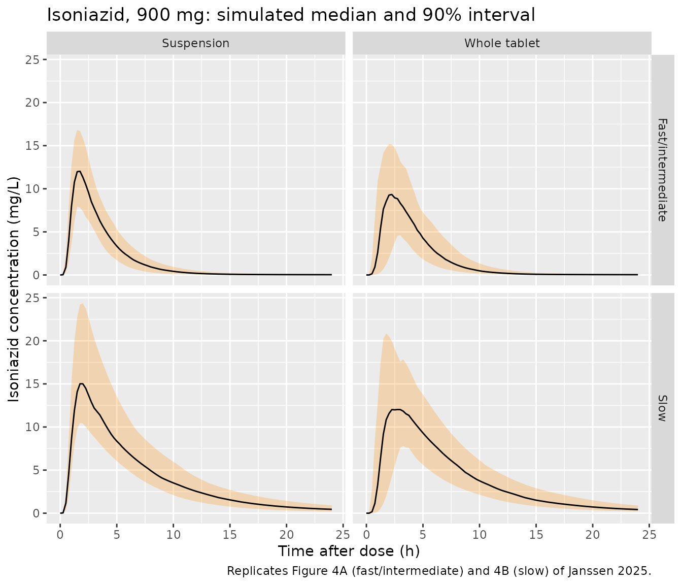
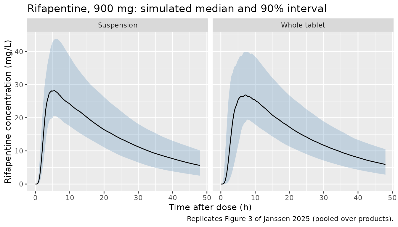
The suspension peaks earlier and less variably for both drugs, as in the paper, while the peak height changes little.
PKNCA validation
NCA uses the protocol sampling times (pre-dose and 1, 2, 3, 4, 5, 6, 8, 24 and 48 h), so that Tmax is read off the same grid as in the study.
run_nca <- function(sim, end) {
  conc <- sim |>
    filter(!is.na(Cc), time %in% grid_protocol, time <= end) |>
    select(id, time, Cc, form)
  conc <- bind_rows(conc, distinct(conc, id, form) |> mutate(time = 0, Cc = 0)) |>
    distinct(id, form, time, .keep_all = TRUE) |>
    arrange(id, form, time)
  dose <- events |>
    filter(evid == 1) |>
    select(id, time, amt, form)
  intervals <- data.frame(start = 0, end = end, cmax = TRUE, tmax = TRUE, auclast = TRUE)
  PKNCA::pk.nca(PKNCA::PKNCAdata(
    PKNCA::PKNCAconc(conc, Cc ~ time | form + id),
    PKNCA::PKNCAdose(dose, amt ~ time | form + id),
    intervals = intervals
  ))
}
nca_rpt <- run_nca(sim_rpt, end = 48)
nca_inh <- run_nca(sim_inh, end = 24)
Comparison against published NCA
Table 3 reports median AUC, Cmax and Tmax for each product and form. The reference below holds all three product rows per form; the comparison table pools them by their median. All rifapentine samples at 168 h were BLQ, so the published AUC0-168 is in effect the area to the last quantifiable sample at 48 h, and is compared with the simulated AUC0-48.
ref_rpt <- tibble::tribble(
  ~form,          ~auclast, ~cmax, ~tmax,
  "Suspension",   705.9,    31.8,  5.49,
  "Suspension",   770.9,    34.1,  5.01,
  "Suspension",   674,      32.85, 5,
  "Whole tablet", 675.9,    30.35, 6,
  "Whole tablet", 708.5,    34.35, 5.05,
  "Whole tablet", 626.9,    30.15, 5.5
)
ref_inh <- tibble::tribble(
  ~form,          ~auclast, ~cmax, ~tmax,
  "Suspension",   43.18,    10.8,  2,
  "Suspension",   50.95,    13.05, 2.49,
  "Suspension",   46.59,    10.75, 2,
  "Whole tablet", 56.61,    13.4,  2.5,
  "Whole tablet", 36.41,    9.78,  2,
  "Whole tablet", 40.83,    12.05, 3
)
units_nca <- c(auclast = "mg*h/L", cmax = "mg/L", tmax = "h")
cmp_rpt <- nlmixr2lib::ncaComparisonTable(
  simulated = nca_rpt, reference = ref_rpt, by = "form",
  units = units_nca, tolerance_pct = 20
)
cmp_inh <- nlmixr2lib::ncaComparisonTable(
  simulated = nca_inh, reference = ref_inh, by = "form",
  units = units_nca, tolerance_pct = 20
)
knitr::kable(cmp_rpt, caption = "Rifapentine: simulated vs Table 3 medians (AUC0-48 vs published AUC0-168). * differs by >20%.")| NCA parameter | form | Reference | Simulated | % diff |
|---|---|---|---|---|
| Cmax (mg/L) | Suspension | 32.8 | 29 | -11.8% |
| Cmax (mg/L) | Whole tablet | 30.4 | 27.9 | -8.2% |
| Tmax (h) | Suspension | 5.01 | 5 | -0.2% |
| Tmax (h) | Whole tablet | 5.5 | 6 | +9.1% |
| AUClast (mg*h/L) | Suspension | 706 | 699 | -1.0% |
| AUClast (mg*h/L) | Whole tablet | 676 | 704 | +4.1% |
knitr::kable(cmp_inh, caption = "Isoniazid: simulated vs Table 3 medians (AUC0-24). * differs by >20%.")| NCA parameter | form | Reference | Simulated | % diff |
|---|---|---|---|---|
| Cmax (mg/L) | Suspension | 10.8 | 12.1 | +11.9% |
| Cmax (mg/L) | Whole tablet | 12 | 11.2 | -7.3% |
| Tmax (h) | Suspension | 2 | 2 | +0.0% |
| Tmax (h) | Whole tablet | 2.5 | 2 | -20.0% |
| AUClast (mg*h/L) | Suspension | 46.6 | 52.9 | +13.6% |
| AUClast (mg*h/L) | Whole tablet | 40.8 | 56.5 | +38.5%* |
The isoniazid whole-tablet AUC0-24 row is starred. Each Table 3 median comes from 16 participants whose acetylator classes split roughly two to one, so the product-level medians scatter widely: the three whole-tablet medians are 36.4, 40.8 and 56.6 mg h/L, and the simulated median lies at the top of that range. The structural check below therefore pools the six published product-by-form medians for each drug and parameter, and compares them with the median over all simulated subjects (bioavailability does not depend on the form in either model).
# Structural check: a mis-transcribed clearance, volume, dose or unit moves
# these medians by tens of percent. Observed while authoring: rifapentine
# Cmax -13%, AUC +2%; isoniazid Cmax +2%, AUC +20% (the pooled published
# medians are themselves medians of n = 16 groups).
sim_med <- function(res, code) {
  x <- as.data.frame(res)
  median(x$PPORRES[x$PPTESTCD == code], na.rm = TRUE)
}
chk <- tibble(
  drug = rep(c("Rifapentine", "Isoniazid"), each = 2),
  parameter = rep(c("cmax", "auclast"), 2),
  simulated = c(
    sim_med(nca_rpt, "cmax"), sim_med(nca_rpt, "auclast"),
    sim_med(nca_inh, "cmax"), sim_med(nca_inh, "auclast")
  ),
  published = c(
    median(ref_rpt$cmax), median(ref_rpt$auclast),
    median(ref_inh$cmax), median(ref_inh$auclast)
  )
) |>
  mutate(pct_diff = 100 * (simulated / published - 1))
knitr::kable(chk, digits = 1, caption = "Median over all simulated subjects vs median of the six Table 3 product-by-form medians.")| drug | parameter | simulated | published | pct_diff |
|---|---|---|---|---|
| Rifapentine | cmax | 28.1 | 32.3 | -13.1 |
| Rifapentine | auclast | 701.9 | 690.9 | 1.6 |
| Isoniazid | cmax | 11.6 | 11.4 | 2.0 |
| Isoniazid | auclast | 53.8 | 44.9 | 19.9 |
Assumptions and deviations
-
Rifapentine MTT. Table 2 prints the rifapentine MTT
as 2.34 h with a 90% CI of 2.54-2.97 h; the point estimate lies outside
its own interval. The final-model control stream (ESM 2) carries
TVMTT = 2.75047, at the centre of that interval, so the model uses 2.75 h. With 2.75 h the typical-value Tmax is 6.3 h (whole) and 5.1 h (suspension), against observed medians of 5.0-6.0 h in Table 3; 2.34 h would give 5.5 h and 4.4 h. -
Table 2 vs control-stream values. The
$THETA/$OMEGAinitial values in ESM 2 and ESM 3 are close to, but not identical with, the Table 2 final estimates (e.g. rifapentine CL/F 1.0192 vs 1.03 L/h). Table 2 is used for every value except the rifapentine MTT above. -
Transit absorption. The streams use the Savic
analytical transit input (
NN= 4 for rifapentine, 5 for isoniazid) into a depot absorbed atKA = KTR. The packaged models write the same system as an explicit chain ofNN + 1transit stages plus an absorption compartment, all atktr, which superposes repeated doses exactly; the mass-balance check above confirms the dose is delivered intact. -
Acetylator mixture. The isoniazid model was fitted
with a NONMEM mixture (no NAT2 genotype was available), which rxode2
cannot express as a latent class. The class is supplied as the covariate
NAT2_SLOW(1 = slow); for a population simulation draw it with probability 1 - 0.659 = 0.341, as done here. The model did not separate fast from intermediate acetylators. -
Isoniazid residual error. ESM 3 fits
log-transformed concentrations with
SD = sqrt(0.208^2 + (0.11 / C)^2)on the log scale. To first order this is a combined proportional (20.8%) and additive (0.11 mg/L) error on the linear scale, which is how it is encoded. - Formulation and brand on bioavailability. The final models share one bioavailability across products and forms. The relative bioavailabilities in the Results and Figure 5 (e.g. rifapentine suspension 110.1% for brand 1) come from log-likelihood profiling of separate models and are not part of the packaged models.
-
IOV. Inter-occasion variability is encoded as four
per-occasion etas selected by
OCC(the four sampled weekly doses), with occasions 2-4 fixed to the occasion-1 variance ($OMEGA ... SAME). rxode2 cannot mu-reference these indicator-weighted etas and warns about it; the warning affects only estimation speed, not simulation.OCCvalues outside 1-4 apply no IOV. In the suspension form the IOV deviation on MTT is multiplied by1 + e_susp_iovmtt, as in the streams. - Rifapentine dose. No dose effect on bioavailability was estimated (only 900 mg was given), so the rifapentine parameters apply to 900 mg.
- Virtual cohort. Fat-free mass is drawn log-normal from the Table 1 median and interquartile range; the paper does not give its distribution. NCA medians pool all simulated subjects per form, whereas Table 3 reports each product separately (n = 16 each); the published values are pooled by their median.