Meropenem (Lee 2021) • nlmixr2lib

Model and source

Citation: Lee DH, Kim HS, Park S, Kim HI, Lee SH, Kim YK. (2021). Population Pharmacokinetics of Meropenem in Critically Ill Korean Patients and Effects of Extracorporeal Membrane Oxygenation. Pharmaceutics 13(11):1861. doi:10.3390/pharmaceutics13111861.
Description: Two-compartment intravenous population PK model for meropenem in critically ill Korean adults, including patients on extracorporeal membrane oxygenation (Lee 2021; n = 26, 8 on ECMO, 125 plasma samples). Total clearance increases linearly with CKD-EPI estimated glomerular filtration rate centred at 91.57 mL/min/1.73 m^2: CL = 6.37 * (1 + 0.00925 * (CRCL - 91.57)) L/h. ECMO support was tested and did not affect any PK parameter. Log-normal IIV on CL, Vc and Vp (none on Q); residual error is a power model whose standard deviation is 0.246 * Cc^0.865. The unbound concentration Cu = fu * Cc (fu = 0.98) drives the fT>MIC targets (40% fT>MIC, 100% fT>MIC, 100% fT>4MIC) of the paper’s Monte Carlo probability-of-target-attainment simulations.
Article: Pharmaceutics 2021;13(11):1861 (open access, PMC8625191)

Meropenem is a carbapenem beta-lactam whose efficacy is driven by the fraction of the dosing interval during which the free concentration exceeds the MIC (%fT>MIC). Lee and colleagues fitted a population PK model to critically ill Korean adults, eight of whom were on extracorporeal membrane oxygenation (ECMO), asked whether ECMO changes meropenem PK (it did not), and then used Monte Carlo simulation to find dosing regimens that reach a 90% probability of target attainment (PTA) across six bands of renal function.

Population

Twenty-six ICU patients were enrolled at Hallym University Sacred Heart Hospital, Anyang, South Korea, between September 2020 and April 2021 (Table 1). Eight received ECMO (seven veno-arterial, one veno-venous) and 18 did not. The ECMO group was younger (median age 64.0 vs 72.0 years) and sicker (APACHE II 21.0 vs 16.0; SOFA 9.50 vs 5.00). Overall 8 of 26 patients were female (4 of 8 on ECMO, 4 of 18 without). Median weight was 63.5 kg on ECMO and 54.4 kg without. Renal function spanned impaired to supranormal: the CKD-EPI eGFR, the covariate retained in the final model, had a median (IQR) of 87.7 (70.0-105) mL/min/1.73 m^2 on ECMO and 91.6 (45.6-103) mL/min/1.73 m^2 without.

Patients received 500 or 1000 mg meropenem as a 30-min IV infusion every 8 or 12 h. Five samples were drawn after the first dose following enrolment and two at steady state. The 125 samples used for estimation were fitted in NONMEM 7.5 with FOCE-I, and 44 further trough and peak samples were used for external validation.

The same information is available programmatically via the model’s population metadata (readModelDb("Lee_2021_meropenem")()$population).

Source trace

The per-parameter origin is recorded as an in-file comment next to each ini() entry in inst/modeldb/specificDrugs/Lee_2021_meropenem.R. The table below collects them in one place for review.

Equation / parameter	Value as published	Value in `ini()`	Source location
`lcl`	theta1 = 6.37 L/h (RSE 7.41%; bootstrap 6.32, 95% CI 5.42-7.23)	`log(6.37)`	Table 2, structural model
`e_crcl_cl`	theta2 = 0.00925 (RSE 10.3%; bootstrap 0.00932, 95% CI 0.00680-0.0110)	`0.00925`	Table 2, structural model
CL covariate form	`CL = theta1 * (1 + theta2 * (CE - 91.57))`, CE = CKD-EPI eGFR	`exp(lcl + etalcl) * (1 + e_crcl_cl * (CRCL - 91.57))`	Table 2, structural-model row
`lvc`	VC = 9.07 L (RSE 12.2%)	`log(9.07)`	Table 2
`lq`	Q = 10.7 L/h (RSE 21.5%)	`log(10.7)`	Table 2
`lvp`	VP = 7.91 L (RSE 13.6%)	`log(7.91)`	Table 2
`etalcl`	IIV CL = 31.4% (RSE 15.8%, shrinkage 3.70%)	`0.0940330` = `log(1 + 0.314^2)`	Table 2
`etalvc`	IIV VC = 43.6% (RSE 22.5%, shrinkage 14.7%)	`0.1740340` = `log(1 + 0.436^2)`	Table 2
`etalvp`	IIV VP = 36.6% (RSE 21.0%, shrinkage 41.3%)	`0.1257124` = `log(1 + 0.366^2)`	Table 2
`propSd`	proportional error 24.6% (RSE 29.3%, shrinkage 24.2%)	`0.246`	Table 2
`powExp`	power parameter 0.865 (RSE 10.0%)	`0.865`	Table 2; Methods 2.5
`fu`	“The parameter f was fixed at 98%”	`fixed(0.98)`	Methods 2.7
`d/dt(central)`, `d/dt(peripheral1)`	two-compartment model with CL, VC, VP, Q	n/a	Results 3.2
`Cc ~ pow(propSd, powExp)`	proportional error with a power parameter for heteroscedasticity	n/a	Methods 2.5; Results 3.2
`Cu <- fu * Cc`	%fT>MIC computed on free drug	n/a	Methods 2.7

Results 3.2 states that IIV was estimated for CL, V1 and V2 only, so q carries no random effect, and no covariance between the random effects is reported.

Simulation setup

mod <- readModelDb("Lee_2021_meropenem")
ini_df <- rxode2::rxode(mod)$iniDf
#> ℹ parameter labels from comments will be replaced by 'label()'
theta <- setNames(ini_df$est, ini_df$name)
omega_sd <- sqrt(theta[c("etalcl", "etalvc", "etalvp")])
omega_sd
#>    etalcl    etalvc    etalvp 
#> 0.3066480 0.4171738 0.3545594

The random effects are drawn with base R (stats::rnorm) and passed to rxSolve() as per-subject columns of the event data with omega = NA. That fixes the virtual patients independently of the rxode2 build, and it lets every regimen below be solved on the same patients, so regimen comparisons are paired.

draw_cohort <- function(n, crcl, seed) {
  set.seed(seed)
  tibble::tibble(
    id     = seq_len(n),
    CRCL   = crcl,
    etalcl = stats::rnorm(n, 0, omega_sd[["etalcl"]]),
    etalvc = stats::rnorm(n, 0, omega_sd[["etalvc"]]),
    etalvp = stats::rnorm(n, 0, omega_sd[["etalvp"]])
  )
}

# Solve one event template for every subject in `cohort`. The etas travel as
# columns of the event data; with omega = NA the solve is deterministic. (Passing
# them through `params =` together with `omega = NA` silently zeroes them, which
# the clearance guard below would catch.)
solve_cohort <- function(cohort, ev_template) {
  ev <- cohort |>
    dplyr::select(id, CRCL, etalcl, etalvc, etalvp) |>
    tidyr::crossing(ev_template) |>
    dplyr::arrange(id, time, dplyr::desc(evid))
  s <- rxode2::rxSolve(mod, events = ev, omega = NA, sigma = NA, keep = "CRCL") |>
    as.data.frame()
  # rxSolve omits the id column for a single-subject solve.
  if (!"id" %in% names(s)) s$id <- cohort$id[1]
  if (dplyr::n_distinct(s$id) != nrow(cohort)) stop("rxSolve dropped subjects")
  # Every patient's clearance must equal the closed form built from its own eta.
  chk <- dplyr::distinct(s, id, cl) |> dplyr::left_join(cohort, by = "id")
  cl_expected <- 6.37 * exp(chk$etalcl) * (1 + 0.00925 * (chk$CRCL - 91.57))
  if (any(abs(chk$cl / cl_expected - 1) > 1e-8)) stop("random effects were not applied")
  if (!all(is.finite(s$Cc))) stop("non-finite concentrations")
  s
}

Typical-value check of the covariate model

The Discussion gives the model-predicted typical values as CL = 6.37 L/h and Vss = VC + VP = 17.0 L. At the centring eGFR of 91.57 mL/min/1.73 m^2 the covariate term is exactly 1. The linear eGFR term also fixes CL at the edges of the simulated renal-function range.

typ_cl <- function(crcl) 6.37 * (1 + 0.00925 * (crcl - 91.57))

one_dose <- tibble::tibble(
  time = c(0, 1), amt = c(1000, NA), dur = c(0.5, NA),
  evid = c(1L, 0L), cmt = "central"
)
typ <- solve_cohort(
  tibble::tibble(id = 1:4, CRCL = c(5, 50, 91.57, 170),
                 etalcl = 0, etalvc = 0, etalvp = 0),
  one_dose
) |>
  dplyr::distinct(id, CRCL, cl, vc, vp, q)
#> ℹ parameter labels from comments will be replaced by 'label()'

typ |>
  dplyr::mutate(`CL expected (L/h)` = typ_cl(CRCL), `Vss (L)` = vc + vp) |>
  dplyr::rename(`eGFR (mL/min/1.73 m^2)` = CRCL, `CL model (L/h)` = cl) |>
  dplyr::select(-id, -vc, -vp, -q) |>
  knitr::kable(digits = 3, caption = "Typical-value clearance across renal function.")

Typical-value clearance across renal function.
eGFR (mL/min/1.73 m^2)	CL model (L/h)	CL expected (L/h)	Vss (L)
5.00	1.269	1.269	16.98
50.00	3.921	3.921	16.98
91.57	6.370	6.370	16.98
170.00	10.991	10.991	16.98


stopifnot(
  all(abs(typ$cl - typ_cl(typ$CRCL)) < 1e-8),
  abs(typ$cl[typ$CRCL == 91.57] - 6.37) < 1e-8,
  abs(typ$vc[1] + typ$vp[1] - 17.0) < 0.05
)

Concentration-time profiles

The first simulated dose, 1 g as a 30-min infusion, is shown for the six renal function bands the paper used for its dose-finding simulations (Methods 2.7). Each band has 200 patients with eGFR drawn uniformly within the band, matching the paper’s uniform covariate distribution. The plotted quantity is the individual prediction Cc, without residual error.

renal_bands <- tibble::tibble(
  band = factor(c("0-10", "10-25", "25-50", "50-90", "90-130", "130-170"),
                levels = c("0-10", "10-25", "25-50", "50-90", "90-130", "130-170")),
  lo   = c(0, 10, 25, 50, 90, 130),
  hi   = c(10, 25, 50, 90, 130, 170)
)
n_per_band <- 200L

cohort <- do.call(dplyr::bind_rows, lapply(seq_len(nrow(renal_bands)), function(i) {
  set.seed(2021 + i)
  crcl <- stats::runif(n_per_band, renal_bands$lo[i], renal_bands$hi[i])
  draw_cohort(n_per_band, crcl, seed = 1861 + i) |>
    dplyr::mutate(band = renal_bands$band[i])
})) |>
  dplyr::mutate(id = dplyr::row_number())

cohort |>
  dplyr::group_by(band) |>
  dplyr::summarise(n = dplyr::n(), `median eGFR` = stats::median(CRCL),
                   `SD etalcl` = stats::sd(etalcl), .groups = "drop") |>
  knitr::kable(digits = 3, caption = "Virtual cohort by renal-function band (eGFR in mL/min/1.73 m^2).")

Virtual cohort by renal-function band (eGFR in mL/min/1.73 m^2).
band	n	median eGFR	SD etalcl
0-10	200	5.592	0.317
10-25	200	17.041	0.308
25-50	200	37.124	0.307
50-90	200	71.535	0.289
90-130	200	107.208	0.305
130-170	200	150.898	0.286

sd_times <- sort(unique(c(seq(0, 1, by = 0.1), seq(1.25, 24, by = 0.25))))
single_ev <- dplyr::bind_rows(
  tibble::tibble(time = 0, amt = 1000, dur = 0.5, evid = 1L, cmt = "central"),
  tibble::tibble(time = sd_times, amt = NA_real_, dur = NA_real_, evid = 0L, cmt = "central")
)
sim_sd <- solve_cohort(cohort, single_ev) |>
  dplyr::left_join(dplyr::select(cohort, id, band), by = "id")

sim_sd |>
  dplyr::filter(time > 0) |>
  dplyr::group_by(band, time) |>
  dplyr::summarise(Q10 = stats::quantile(Cc, 0.10), Q50 = stats::median(Cc),
                   Q90 = stats::quantile(Cc, 0.90), .groups = "drop") |>
  ggplot2::ggplot(ggplot2::aes(time, Q50)) +
  ggplot2::geom_ribbon(ggplot2::aes(ymin = Q10, ymax = Q90), alpha = 0.25) +
  ggplot2::geom_line() +
  ggplot2::facet_wrap(~band, labeller = ggplot2::label_both) +
  ggplot2::scale_y_log10() +
  ggplot2::labs(x = "Time after start of infusion (h)",
                y = "Meropenem Cc (mg/L)",
                title = "Single 1 g 30-min infusion: median and 10th-90th percentile",
                caption = "Model-side analogue of the Lee 2021 Figure 2 VPC (which pools all doses).")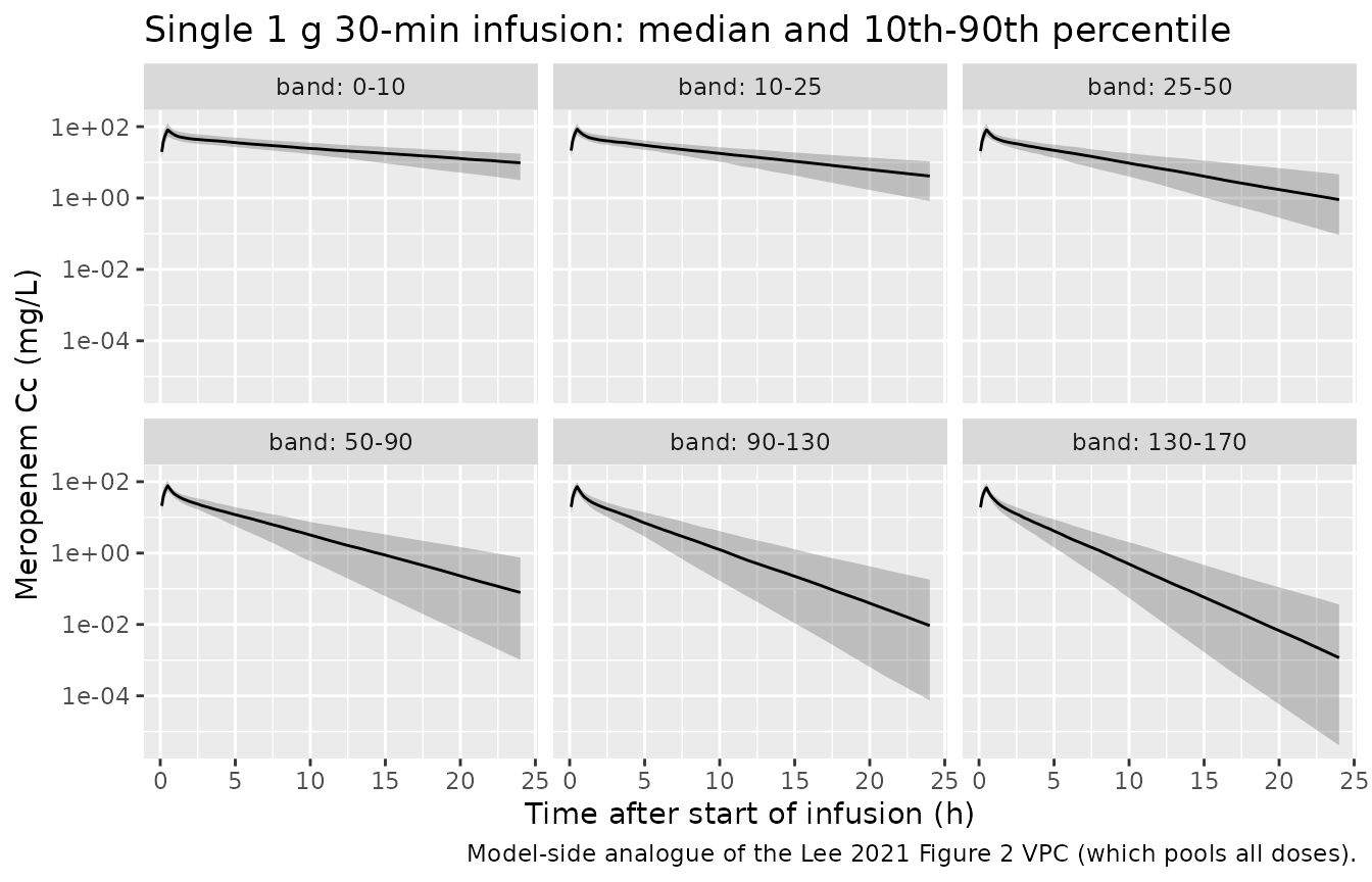

PKNCA validation

The paper reports no NCA table, so the NCA here checks the model against its own exact identities. For a linear model with IV input, AUCinf = Dose / CL, so the NCA clearance per subject must equal the model clearance, and the NCA Vss must equal vc + vp.

# A sparse, clinically realistic grid keeps the NCA fast; the dense grid above
# is for the figure only.
nca_times <- c(0, 0.5, 1, 1.5, 2, 3, 4, 6, 8, 10, 12, 16, 20, 24)
sim_nca <- solve_cohort(cohort, dplyr::bind_rows(
  tibble::tibble(time = 0, amt = 1000, dur = 0.5, evid = 1L, cmt = "central"),
  tibble::tibble(time = nca_times, amt = NA_real_, dur = NA_real_, evid = 0L, cmt = "central")
)) |>
  dplyr::left_join(dplyr::select(cohort, id, band), by = "id")

nca_conc <- sim_nca |>
  dplyr::filter(!is.na(Cc)) |>
  dplyr::mutate(treatment = factor(paste("eGFR", band),
                                   levels = paste("eGFR", levels(band)))) |>
  dplyr::select(id, time, Cc, treatment)

# An IV pre-dose concentration is zero; guarantee a time-zero record.
nca_conc <- dplyr::bind_rows(
  nca_conc,
  nca_conc |> dplyr::distinct(id, treatment) |> dplyr::mutate(time = 0, Cc = 0)
) |>
  dplyr::distinct(id, treatment, time, .keep_all = TRUE) |>
  dplyr::arrange(id, treatment, time)

nca_dose <- nca_conc |>
  dplyr::distinct(id, treatment) |>
  dplyr::mutate(time = 0, amt = 1000, dur = 0.5)

intervals <- data.frame(
  start = 0, end = Inf,
  cmax = TRUE, tmax = TRUE, auclast = TRUE, aucinf.obs = TRUE,
  half.life = TRUE, cl.obs = TRUE, vss.iv.obs = TRUE
)
# One pk.nca() call per band: a single call over all 1,200 subjects is far
# slower than six calls of 200.
nca_res <- do.call(dplyr::bind_rows, lapply(unique(nca_conc$treatment), function(trt) {
  res <- PKNCA::pk.nca(PKNCA::PKNCAdata(
    PKNCA::PKNCAconc(dplyr::filter(nca_conc, treatment == trt), Cc ~ time | treatment + id,
                     concu = "mg/L", timeu = "h"),
    PKNCA::PKNCAdose(dplyr::filter(nca_dose, treatment == trt), amt ~ time | treatment + id,
                     doseu = "mg", route = "intravascular", duration = "dur"),
    intervals = intervals
  ))
  as.data.frame(res)
}))

nca_wide <- nca_res |>
  dplyr::filter(PPTESTCD %in% c("cmax", "aucinf.obs", "half.life", "cl.obs", "vss.iv.obs")) |>
  dplyr::select(id, treatment, PPTESTCD, PPORRES) |>
  tidyr::pivot_wider(names_from = PPTESTCD, values_from = PPORRES)

nca_wide |>
  dplyr::group_by(treatment) |>
  dplyr::summarise(dplyr::across(c(cmax, aucinf.obs, half.life, cl.obs, vss.iv.obs),
                                 stats::median), .groups = "drop") |>
  dplyr::rename(`Renal band` = treatment, `Cmax (mg/L)` = cmax,
                `AUC0-inf (mg*h/L)` = aucinf.obs, `t1/2 (h)` = half.life,
                `CL (L/h)` = cl.obs, `Vss (L)` = vss.iv.obs) |>
  knitr::kable(digits = 2, caption = "Median NCA parameters after a single 1 g 30-min infusion, by eGFR band.")

Median NCA parameters after a single 1 g 30-min infusion, by eGFR band.
Renal band	Cmax (mg/L)	AUC0-inf (mg*h/L)	t1/2 (h)	CL (L/h)	Vss (L)
eGFR 0-10	81.56	758.94	10.06	1.32	18.22
eGFR 10-25	85.12	512.31	6.47	1.95	17.78
eGFR 25-50	81.39	321.63	4.23	3.11	18.14
eGFR 50-90	76.80	184.25	2.60	5.43	17.74
eGFR 90-130	72.99	135.90	1.97	7.36	18.30
eGFR 130-170	67.83	97.97	1.58	10.21	19.48

ident <- nca_wide |>
  dplyr::left_join(dplyr::distinct(sim_nca, id, cl, vc, vp), by = "id") |>
  dplyr::mutate(cl_ratio = cl.obs / cl, vss_ratio = vss.iv.obs / (vc + vp))

ident |>
  dplyr::group_by(treatment) |>
  dplyr::summarise(`median NCA CL / model CL` = stats::median(cl_ratio),
                   `median NCA Vss / model Vss` = stats::median(vss_ratio),
                   .groups = "drop") |>
  dplyr::rename(`Renal band` = treatment) |>
  knitr::kable(digits = 4, caption = "NCA recovers the model clearance and steady-state volume.")

NCA recovers the model clearance and steady-state volume.
Renal band	median NCA CL / model CL	median NCA Vss / model Vss
eGFR 0-10	1.0010	1.0008
eGFR 10-25	1.0013	1.0026
eGFR 25-50	1.0022	1.0065
eGFR 50-90	1.0058	1.0191
eGFR 90-130	1.0087	1.0307
eGFR 130-170	1.0141	1.0504


# Both sides use the same drawn parameters; the residual is the trapezoid and
# the log-linear extrapolation beyond 24 h, which is largest in the lowest band.
stopifnot(
  abs(stats::median(ident$cl_ratio) - 1) < 0.02,
  abs(stats::median(ident$vss_ratio) - 1) < 0.05
)

Comparison against the published typical values

The only cohort-level PK summaries in the paper are the Discussion’s typical values (CL 6.37 L/h, Vss 17.0 L). They are compared below with the PKNCA estimates for a single typical patient at the centring eGFR of 91.57 mL/min/1.73 m^2.

typ_ev <- tibble::tibble(
  time = c(0, sd_times[sd_times > 0], 36, 48), amt = c(1000, rep(NA, sum(sd_times > 0) + 2)),
  dur = c(0.5, rep(NA, sum(sd_times > 0) + 2)),
  evid = c(1L, rep(0L, sum(sd_times > 0) + 2)), cmt = "central"
)
typ_sim <- solve_cohort(
  tibble::tibble(id = 1L, CRCL = 91.57, etalcl = 0, etalvc = 0, etalvp = 0),
  typ_ev
) |>
  dplyr::mutate(treatment = "Typical patient, eGFR 91.57")

typ_conc <- dplyr::bind_rows(
  dplyr::select(typ_sim, id, time, Cc, treatment),
  tibble::tibble(id = 1L, time = 0, Cc = 0, treatment = "Typical patient, eGFR 91.57")
) |>
  dplyr::distinct(id, treatment, time, .keep_all = TRUE) |>
  dplyr::arrange(time)

typ_nca <- PKNCA::pk.nca(PKNCA::PKNCAdata(
  PKNCA::PKNCAconc(typ_conc, Cc ~ time | treatment + id, concu = "mg/L", timeu = "h"),
  PKNCA::PKNCAdose(
    tibble::tibble(id = 1L, time = 0, amt = 1000, dur = 0.5,
                   treatment = "Typical patient, eGFR 91.57"),
    amt ~ time | treatment + id, doseu = "mg", route = "intravascular", duration = "dur"
  ),
  intervals = data.frame(start = 0, end = Inf, aucinf.obs = TRUE, cl.obs = TRUE,
                         vss.iv.obs = TRUE)
))

published <- tibble::tibble(
  treatment = "Typical patient, eGFR 91.57",
  aucinf.obs = 1000 / 6.37, cl.obs = 6.37, vss.iv.obs = 17.0
)

cmp <- nlmixr2lib::ncaComparisonTable(
  simulated = typ_nca,
  reference = published,
  by = "treatment",
  units = c(aucinf.obs = "mg*h/L", cl.obs = "L/h", vss.iv.obs = "L"),
  tolerance_pct = 20
)
knitr::kable(cmp, caption = paste(
  "Simulated typical patient vs. the Lee 2021 Discussion typical values",
  "(AUC0-inf reference = 1000 mg / 6.37 L/h). * differs from reference by >20%."
))

Simulated typical patient vs. the Lee 2021 Discussion typical values (AUC0-inf reference = 1000 mg / 6.37 L/h). * differs from reference by >20%.
NCA parameter	treatment	Reference	Simulated	% diff
AUC0-∞ (obs) (mg*h/L)	Typical patient, eGFR 91.57	157	157	+0.0%
CL/F (L/h)	Typical patient, eGFR 91.57	6.37	6.37	-0.0%
Vss (IV) (L)	Typical patient, eGFR 91.57	17	17	-0.1%


typ_wide <- as.data.frame(typ_nca) |>
  dplyr::select(PPTESTCD, PPORRES) |>
  tidyr::pivot_wider(names_from = PPTESTCD, values_from = PPORRES)
stopifnot(
  abs(typ_wide$cl.obs / 6.37 - 1) < 0.01,
  abs(typ_wide$vss.iv.obs / 17.0 - 1) < 0.02
)

Table 3 of the paper also gives the medians (IQR) of the individual (empirical-Bayes) estimates by group: CL 6.34 L/h on ECMO and 5.05 L/h without, and Vss 16.2 L and 17.2 L. The model’s typical CL at each group’s median eGFR from Table 1 is 6.14 L/h (ECMO, 87.7) and 6.37 L/h (non-ECMO, 91.6). The ECMO value agrees. The non-ECMO median of the individual estimates is about 20% lower. The individual CL values are not published, so this gap cannot be traced further; the typical value is what the paper’s own simulations used.

Probability of target attainment

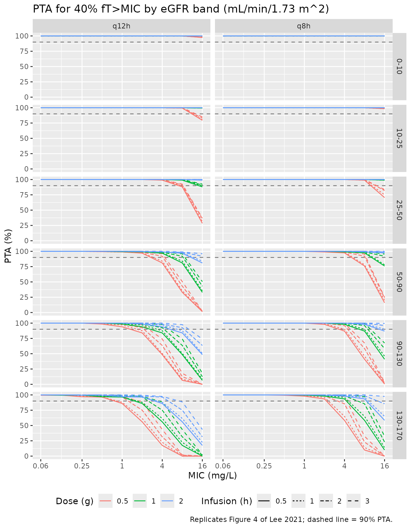
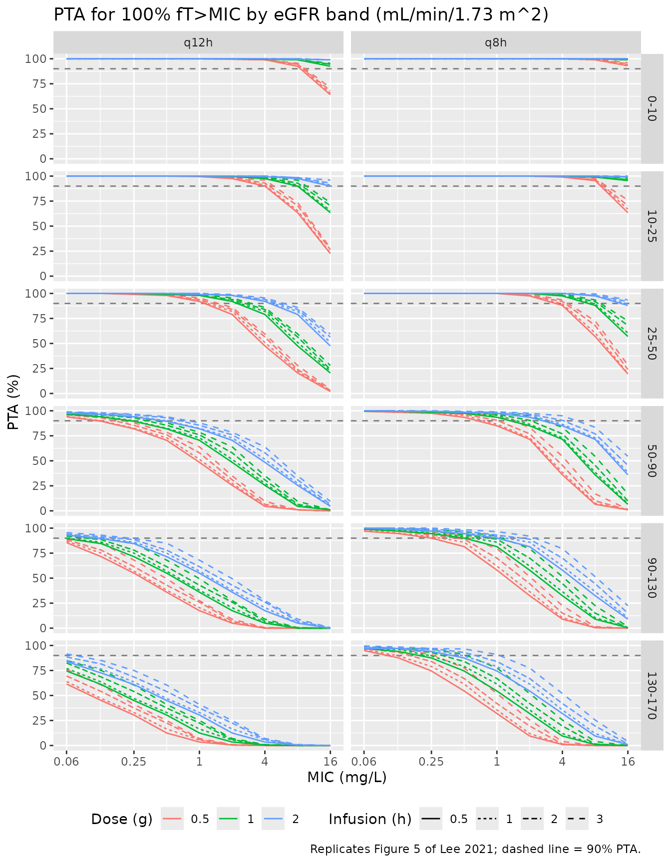
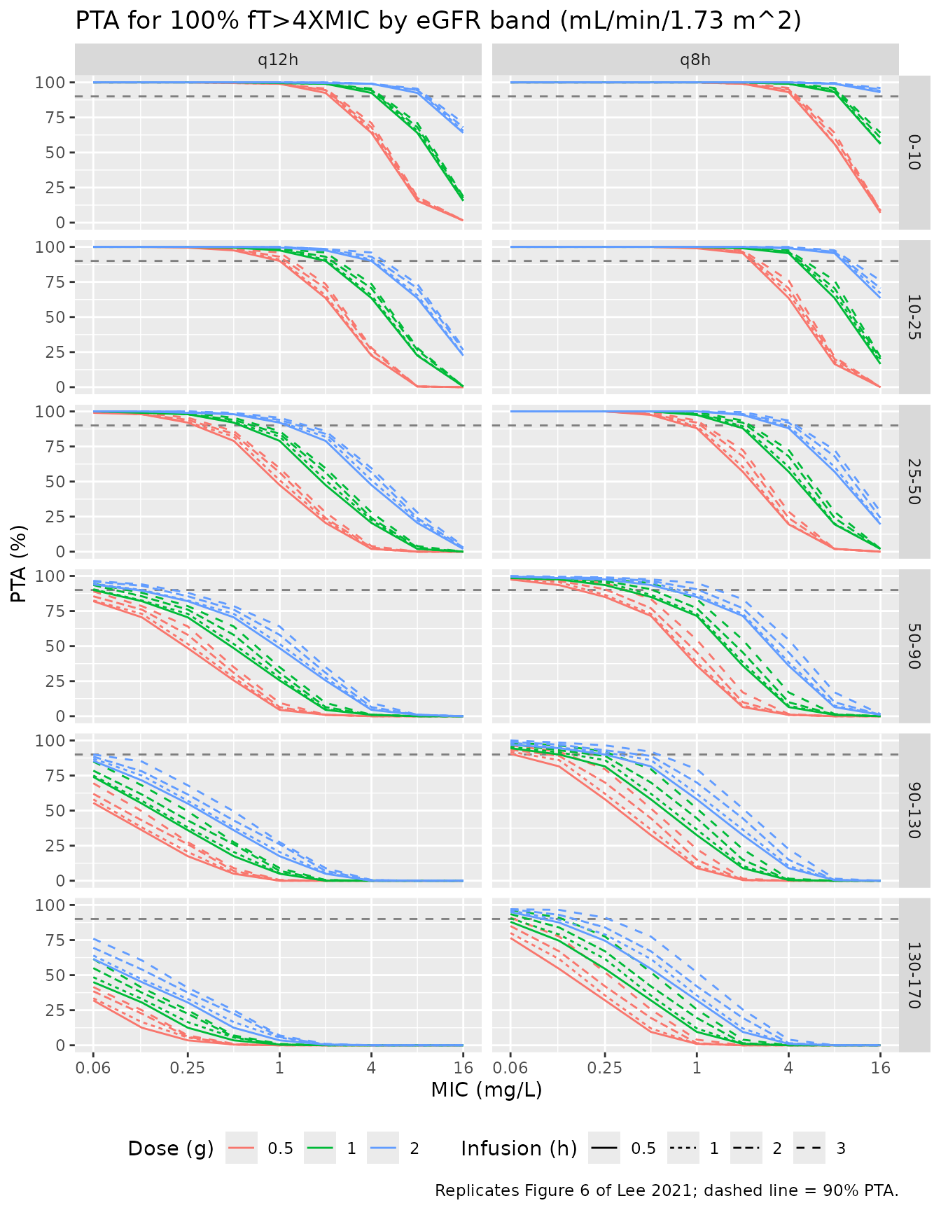
Methods 2.7 describes the dose-finding simulations. Virtual patients were given uniformly distributed eGFR between 0 and 170 mL/min/1.73 m^2 and split into six renal bands. Each received every combination of three doses (0.5, 1 and 2 g), two dosing intervals (8 and 12 h) and four infusion durations (0.5, 1, 2 and 3 h) at steady state. The PTA was computed for three targets on the free concentration (fu = 0.98): 40% fT>MIC (Figure 4), 100% fT>MIC (Figure 5) and 100% fT>4XMIC (Figure 6). A regimen is adequate when the PTA is at least 90%.

Steady state is solved directly with ss = 1. Because the model is linear, a 0.5 g or 2 g profile is exactly 0.5 or 2 times the 1 g profile of the same patient. So only the eight interval-by-infusion shapes need solving, each at 1 g, over the cohort of 1,200 patients (200 per band).

shapes <- tidyr::expand_grid(tau = c(8, 12), dur = c(0.5, 1, 2, 3))
dt <- 0.05

ss_profiles <- do.call(dplyr::bind_rows, lapply(seq_len(nrow(shapes)), function(i) {
  tau <- shapes$tau[i]; dur <- shapes$dur[i]
  ev <- dplyr::bind_rows(
    tibble::tibble(time = 0, amt = 1000, dur = dur, ii = tau, ss = 1L,
                   evid = 1L, cmt = "central"),
    tibble::tibble(time = seq(0, tau - dt, by = dt), amt = NA_real_,
                   dur = NA_real_, ii = NA_real_, ss = NA_integer_,
                   evid = 0L, cmt = "central")
  )
  solve_cohort(cohort, ev) |>
    dplyr::select(id, time, Cu, cl) |>
    dplyr::mutate(tau = tau, dur = dur)
}))

Two structural gates come before any PTA is read. First, the steady-state interval must satisfy AUCtau = Dose / CL for every patient; both sides use the same drawn parameters, so the tolerance is tight. Second, ss = 1 must agree with an explicit 20-dose train at the slowest clearance simulated, where steady state takes longest to reach.

auc_gate <- ss_profiles |>
  dplyr::group_by(id, tau, dur) |>
  dplyr::summarise(auc = sum(Cu) * dt / 0.98, cl = cl[1], .groups = "drop") |>
  dplyr::mutate(ratio = auc / (1000 / cl))
stopifnot(all(abs(auc_gate$ratio - 1) < 0.01))

slow <- tibble::tibble(id = 1L, CRCL = 0, etalcl = 0, etalvc = 0, etalvp = 0)
tr_ev <- dplyr::bind_rows(
  tibble::tibble(time = seq(0, 19 * 12, by = 12), amt = 1000, dur = 0.5, evid = 1L, cmt = "central"),
  tibble::tibble(time = 19 * 12 + c(0, 0.5, 6), amt = NA_real_, dur = NA_real_,
                 evid = 0L, cmt = "central")
)
tr <- solve_cohort(slow, tr_ev) |> dplyr::filter(time >= 19 * 12)
ss_ev <- dplyr::bind_rows(
  tibble::tibble(time = 0, amt = 1000, dur = 0.5, ii = 12, ss = 1L, evid = 1L, cmt = "central"),
  tibble::tibble(time = c(0, 0.5, 6), amt = NA_real_, dur = NA_real_, ii = NA_real_,
                 ss = NA_integer_, evid = 0L, cmt = "central")
)
ss1 <- solve_cohort(slow, ss_ev)
stopifnot(all(abs(tr$Cc / ss1$Cc - 1) < 1e-3))

mics <- c(0.06, 0.125, 0.25, 0.5, 1, 2, 4, 8, 16)
targets <- tibble::tibble(
  target = c("40% fT>MIC", "100% fT>MIC", "100% fT>4XMIC"),
  mult   = c(1, 1, 4),
  frac   = c(0.40, 1, 1)
)

# Every (dose, MIC, target) reduces to one threshold on the 1 g profile:
# dose_g * Cu > mult * MIC  <=>  Cu > mult * MIC / dose_g.
thr_grid <- tidyr::expand_grid(dose_g = c(0.5, 1, 2), MIC = mics, targets) |>
  dplyr::mutate(eff = mult * MIC / dose_g)

# Per patient and shape, %fT>threshold is 1 - ECDF(threshold) over the
# equally spaced steady-state grid; findInterval() gives all thresholds at once.
prof_keys <- dplyr::distinct(ss_profiles, id, tau, dur)
prof_split <- split(ss_profiles$Cu, list(ss_profiles$id, ss_profiles$tau, ss_profiles$dur),
                    drop = TRUE)
prof_split <- prof_split[paste(prof_keys$id, prof_keys$tau, prof_keys$dur, sep = ".")]
ft_mat <- vapply(prof_split, function(cu) {
  1 - findInterval(thr_grid$eff, sort(cu)) / length(cu)
}, numeric(nrow(thr_grid)))

ft <- prof_keys[rep(seq_len(nrow(prof_keys)), each = nrow(thr_grid)), ] |>
  dplyr::bind_cols(thr_grid[rep(seq_len(nrow(thr_grid)), times = nrow(prof_keys)), ]) |>
  dplyr::mutate(ft = as.vector(ft_mat))

pta <- ft |>
  dplyr::left_join(dplyr::select(cohort, id, band), by = "id") |>
  dplyr::group_by(band, tau, dur, dose_g, MIC, target) |>
  dplyr::summarise(PTA = 100 * mean(ft >= frac - 1e-9), .groups = "drop") |>
  dplyr::mutate(regimen = sprintf("%g g q%gh, %g-h", dose_g, tau, dur))

plot_pta <- function(tgt, fig) {
  pta |>
    dplyr::filter(target == tgt) |>
    dplyr::mutate(interval = paste0("q", tau, "h")) |>
    ggplot2::ggplot(ggplot2::aes(MIC, PTA, colour = factor(dose_g),
                                 linetype = factor(dur))) +
    ggplot2::geom_hline(yintercept = 90, colour = "grey50", linetype = "dashed") +
    ggplot2::geom_line() +
    ggplot2::facet_grid(band ~ interval) +
    ggplot2::scale_x_log10(breaks = c(0.06, 0.25, 1, 4, 16),
                           labels = c("0.06", "0.25", "1", "4", "16")) +
    ggplot2::labs(x = "MIC (mg/L)", y = "PTA (%)", colour = "Dose (g)",
                  linetype = "Infusion (h)",
                  title = paste("PTA for", tgt, "by eGFR band (mL/min/1.73 m^2)"),
                  caption = paste("Replicates Figure", fig, "of Lee 2021; dashed line = 90% PTA.")) +
    ggplot2::theme(legend.position = "bottom")
}

Figure 4 – 40% fT>MIC

plot_pta("40% fT>MIC", 4)

Figure 5 – 100% fT>MIC

plot_pta("100% fT>MIC", 5)

Figure 6 – 100% fT>4XMIC

plot_pta("100% fT>4XMIC", 6)

The published dose-finding claims

Results 3.4 makes twelve specific statements about Figures 4-6. Each is stated below as the highest MIC at which the regimen reaches 90% PTA (the “PTA breakpoint”), compared with the simulated breakpoint on the same two-fold MIC grid. The claim is reproduced when the simulated breakpoint satisfies the published relation.

A PTA breakpoint is a tail quantity: it is set by the 10% of patients with the fastest elimination. With 200 patients per band, a PTA near 90% carries a Monte Carlo standard error of about 2 percentage points, so a regimen that sits on the boundary can move one MIC dilution. The assertion therefore requires every claim to hold within one dilution. Exact agreement is reported per claim.

bp <- function(tgt, band_lbl, dose, tau, dur) {
  x <- pta[pta$target == tgt & pta$band == band_lbl & pta$dose_g == dose &
             pta$tau == tau & pta$dur == dur, ]
  ok <- x$MIC[x$PTA >= 90]
  if (length(ok) == 0) 0 else max(ok)
}

claims <- tibble::tribble(
  ~figure, ~target,         ~band,     ~dose, ~tau, ~dur, ~rel, ~mic, ~text,
  4, "40% fT>MIC",    "25-50",   1,     12,   0.5,  ">=", 4,    "1 g q12h 30-min attains 90% PTA at MIC 4",
  4, "40% fT>MIC",    "25-50",   0.5,   12,   0.5,  ">=", 4,    "0.5 g q12h also appropriate (MIC 4)",
  4, "40% fT>MIC",    "90-130",  1,     12,   2,    ">=", 4,    "1 g q12h 2-h infusion optimum at MIC 4",
  4, "40% fT>MIC",    "90-130",  1,     12,   0.5,  "<",  4,    "1 g q12h 30-min does not reach MIC 4",
  4, "40% fT>MIC",    "90-130",  1,     12,   1,    "<",  4,    "1 g q12h 1-h does not reach MIC 4",
  5, "100% fT>MIC",   "50-90",   1,     8,    0.5,  "==", 1,    "1 g q8h 30-min: 90% PTA at MIC 1",
  5, "100% fT>MIC",   "50-90",   1,     8,    3,    "==", 2,    "1 g q8h 3-h: 90% PTA at MIC 2",
  5, "100% fT>MIC",   "130-170", 1,     8,    3,    "==", 0.25, "1 g q8h 3-h: only MIC <= 0.25",
  5, "100% fT>MIC",   "130-170", 2,     8,    3,    "==", 0.5,  "2 g q8h 3-h: MIC < 1",
  6, "100% fT>4XMIC", "50-90",   1,     8,    0.5,  "==", 0.25, "1 g q8h 30-min: MIC <= 0.25",
  6, "100% fT>4XMIC", "50-90",   2,     8,    3,    "==", 1,    "2 g q8h 3-h: MIC <= 1",
  6, "100% fT>4XMIC", "130-170", 2,     8,    3,    "==", 0.125, "2 g q8h 3-h: MIC < 0.25"
)

claims$sim_bp <- vapply(seq_len(nrow(claims)), function(i) {
  with(claims[i, ], bp(target, band, dose, tau, dur))
}, numeric(1))

# log2 distance from the published relation (0 when it holds exactly).
claims <- claims |>
  dplyr::mutate(
    l2 = log2(pmax(sim_bp, 0.03) / mic),
    exact = dplyr::case_when(
      rel == ">=" ~ sim_bp >= mic,
      rel == "<"  ~ sim_bp < mic,
      TRUE        ~ sim_bp == mic
    ),
    miss_dil = dplyr::case_when(
      rel == ">=" ~ pmax(0, -l2),
      rel == "<"  ~ pmax(0, l2 + 1),
      TRUE        ~ abs(l2)
    )
  )

claims |>
  dplyr::transmute(Figure = figure, Target = target, `eGFR band` = band,
                   Claim = text,
                   `Published breakpoint` = paste(rel, mic),
                   `Simulated breakpoint (mg/L)` = sim_bp,
                   `Exact` = exact,
                   `Dilutions off` = round(miss_dil, 2)) |>
  knitr::kable(caption = "Lee 2021 Results 3.4 dose-finding claims vs. simulation.")

Lee 2021 Results 3.4 dose-finding claims vs. simulation.
Figure	Target	eGFR band	Claim	Published breakpoint	Simulated breakpoint (mg/L)	Exact	Dilutions off
4	40% fT>MIC	25-50	1 g q12h 30-min attains 90% PTA at MIC 4	>= 4	8.00	TRUE	0
4	40% fT>MIC	25-50	0.5 g q12h also appropriate (MIC 4)	>= 4	4.00	TRUE	0
4	40% fT>MIC	90-130	1 g q12h 2-h infusion optimum at MIC 4	>= 4	4.00	TRUE	0
4	40% fT>MIC	90-130	1 g q12h 30-min does not reach MIC 4	< 4	2.00	TRUE	0
4	40% fT>MIC	90-130	1 g q12h 1-h does not reach MIC 4	< 4	2.00	TRUE	0
5	100% fT>MIC	50-90	1 g q8h 30-min: 90% PTA at MIC 1	== 1	1.00	TRUE	0
5	100% fT>MIC	50-90	1 g q8h 3-h: 90% PTA at MIC 2	== 2	2.00	TRUE	0
5	100% fT>MIC	130-170	1 g q8h 3-h: only MIC <= 0.25	== 0.25	0.50	FALSE	1
5	100% fT>MIC	130-170	2 g q8h 3-h: MIC < 1	== 0.5	1.00	FALSE	1
6	100% fT>4XMIC	50-90	1 g q8h 30-min: MIC <= 0.25	== 0.25	0.25	TRUE	0
6	100% fT>4XMIC	50-90	2 g q8h 3-h: MIC <= 1	== 1	1.00	TRUE	0
6	100% fT>4XMIC	130-170	2 g q8h 3-h: MIC < 0.25	== 0.125	0.25	FALSE	1


stopifnot(all(claims$miss_dil <= 1 + 1e-9))

9 of the 12 claims reproduce exactly, and all 12 hold within one MIC dilution.

The augmented-renal-clearance claims are one knife-edge inequality

The claims that miss by a dilution are all in the 130-170 mL/min/1.73 m^2 band on the q8h 3-h infusion: 1 g for 100% fT>MIC at MIC 0.5, 2 g for 100% fT>MIC at MIC 1, and 2 g for 100% fT>4XMIC at MIC 0.25. Because the model is linear, all three are the same inequality: the steady-state free trough of the 1 g profile must exceed 0.5 mg/L. The paper places all three just below 90% PTA. The simulation places them at the value below, from the same 200 patients.

arc_pta <- ft |>
  dplyr::left_join(dplyr::select(cohort, id, band), by = "id") |>
  dplyr::filter(band == "130-170", tau == 8, dur == 3) |>
  dplyr::semi_join(
    tibble::tribble(
      ~dose_g, ~MIC, ~target,
      1,       0.5,  "100% fT>MIC",
      2,       1,    "100% fT>MIC",
      2,       0.25, "100% fT>4XMIC"
    ),
    by = c("dose_g", "MIC", "target")
  ) |>
  dplyr::group_by(dose_g, MIC, target) |>
  dplyr::summarise(PTA = 100 * mean(ft >= frac - 1e-9), .groups = "drop")

arc_pta |>
  dplyr::rename(`Dose (g)` = dose_g, `MIC (mg/L)` = MIC, Target = target,
                `Simulated PTA (%)` = PTA) |>
  knitr::kable(caption = "eGFR 130-170, q8h 3-h infusion: three claims, one threshold (0.5 mg/L per g).")

eGFR 130-170, q8h 3-h infusion: three claims, one threshold (0.5 mg/L per g).
Dose (g)	MIC (mg/L)	Target	Simulated PTA (%)
1	0.50	100% fT>MIC	91
2	0.25	100% fT>4XMIC	91
2	1.00	100% fT>MIC	91


# All three rows are one inequality on the same patients, so they must agree.
stopifnot(nrow(arc_pta) == 3L, dplyr::n_distinct(arc_pta$PTA) == 1L)

A PTA this close to 90% is below the resolution of either simulation. The binomial standard error at 90% is about 2.1 points with 200 patients per band, and about 2.3 points for the paper’s roughly 170 patients per band (1,000 patients over six bands). The disagreement is therefore within Monte Carlo error. It does not point to a difference in the model.

Assumptions and deviations

Interindividual-variability scale. Table 2 reports the IIV magnitudes as bare percentages (31.4%, 43.6%, 36.6%) under an exponential random-effect model (theta_i = theta * exp(eta_i)). It does not say whether each is sqrt(omega^2) * 100 or the log-normal sqrt(exp(omega^2) - 1) * 100. The package convention omega^2 = log(CV^2 + 1) is used. The two readings differ by under 4% on the standard deviation (0.3067 vs 0.314 for the CL eta).
Power residual-error model. Table 2 lists “Proportional error 24.6%” and “Power parameter 0.865”. Methods 2.5 says the power parameter was added to “allow for nonlinear heteroscedastic variances”. This is encoded as Cc ~ pow(propSd, powExp), i.e. SD = 0.246 * Cc^0.865. The paper prints no control stream, so the exact NONMEM $ERROR coding is not confirmed.
Which CKD-EPI eGFR. The paper screened both the BSA-normalized CKD-EPI eGFR (mL/min/1.73 m^2) and a “modified” BSA-de-normalized form (mL/min). The covariate is taken to be the BSA-normalized form (CRCL). The 91.57 centring value lies between that form’s group medians (87.7 and 91.6; Table 1) but above both medians of the modified form (82.4 and 77.7), and the PTA figures label their eGFR bands in mL/min/1.73 m^2.
Renal-band edges. Methods 2.7 defines the bands as 0-10, 10-25, 25-50, 50-90, 90-130 and 130-170. Results 3.4 describes some of them as 26-50 and 50-90 mL/min/1.73 m^2. The Methods edges are used.
First simulation not reproduced. Figure 3 (the empirical-therapy simulation with a CLCR-adjusted label regimen, the EUCAST P. aeruginosa MIC distribution and a log-normal eGFR “within the range of 0 to 130”) is not replicated. The mean and SD of that eGFR distribution and the MIC-distribution frequencies are not given in the paper.
Cohort size and PTA resolution. 200 patients per renal band, the nlmixr2lib vignette cap, against the paper’s 1,000 overall. The claim check therefore allows one MIC dilution per claim (see above). No parameter was adjusted to match any claim.
Individual-estimate medians (Table 3). The non-ECMO median of the individual CL estimates (5.05 L/h) is about 20% below the typical CL at that group’s median eGFR. The paper does not publish the individual estimates or the per-patient eGFR, so this cannot be traced. The model reproduces the Discussion’s typical CL (6.37 L/h) and Vss (17.0 L) exactly.
Typographical inconsistencies in the source. Results 3.2 prints the two-compartment base-model OFV as 6540.693; it is evidently 640.693, since the one- and three-compartment values are 689.840 and 640.694. Results 3.1 says one of the eight ECMO patients received CRRT, but Table 1 lists 3 of 8. Results 3.1 gives ages in “days”; Table 1 gives years. Table 1 prints cystatin C in mg/dL at values (medians 1.34-1.48) typical of mg/L. None of these affects the model.
ECMO. ECMO status, ECMO type and ECMO flow rate were screened and not retained, so the model has no ECMO covariate. It applies equally to patients with and without ECMO, as the paper concludes.
Residual error in simulations. The PTA and NCA simulations use the individual predictions without residual error, matching the paper’s Monte Carlo design (individual PK parameters only).